MegEngine implements convolutional neural network

What this tutorial covers

• Understand the 3-channel color image and the corresponding Tensor representation, and understand the Tensor memory layout form;

• Combined with traditional domain knowledge of computer vision, use 2D convolution operator in neural network;

• According to the previous introduction, use MegEngine to implement convolutional neural network to complete the CIFAR-10 image classification task.

Warning

Starting from this tutorial, the model is more complex, and the amount of computation during training will become huge. It is recommended to use the GPU environment to run the code.

Get the original dataset

The CIFAR-10 dataset is the same as MNIST, you can get：directly through data.dataset

from megengine.data.dataset import CIFAR10
from os.path import expanduser

DATA_PATH = expanduser("~/data/datasets/CIFAR10")

train_dataset = CIFAR10(DATA_PATH, train=True)
test_dataset = CIFAR10(DATA_PATH, train=False)

Similar to the processing of MNIST, the divided training set and test set are obtained here, and they are encapsulated into the Dataset type in MegEngine. For the convenience of analysis, we convert them into NumPy’s ndarray data format：

import numpy as np

X_train, y_train = map(np.array, train_dataset[:])

>>> print(X_train.shape, y_train.shape)
(50000, 32, 32, 3) (50000,)

Learn about dataset information

It can be found that the shape of each image sample in CIFAR-10 is \((32, 32, 3)\), and the height, height, and * of samples with shape \((28, 28, 1)\) in the MNIST dataset Channels* vary in number, let’s learn more about CIFAR-10 sample information：

CIFAR-10 数据集

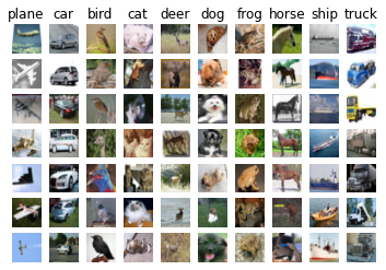
The CIFAR-10 [1] dataset contains 60,000 32x32 color images in a total of 10 categories, each category contains 6,000 images, corresponding to 50,000 training images and 10,000 test images.

Let’s first try to sample each class and visualize it (this code is similar to the MNIST tutorial)：

import cv2
import matplotlib.pyplot as plt

classes = ['plane', 'car', 'bird', 'cat', 'deer',
           'dog', 'frog', 'horse', 'ship', 'truck']
num_classes = len(classes)
samples_per_class = 7

for y, cls in enumerate(classes):
   idxs = np.squeeze(np.where(y_train == y))
   idxs = np.random.choice(idxs, samples_per_class, replace=False)
   for i, idx in enumerate(idxs):
      plt_idx = i * num_classes + y + 1
      plt.subplot(samples_per_class, num_classes, plt_idx)
      plt.imshow(cv2.cvtColor(X_train[idx], cv2.COLOR_BGR2RGB))
      plt.axis('off')
      if i == 0:
            plt.title(cls)
plt.show()

We can do exploratory analysis on the CIFAR-10 dataset in Google’s Know Your Data just like MNIST.

为什么需要使用 cv2.cvtColor 改变颜色（OpenCV）

In the above visualization code, we use the Python interface of OpenCV to change the color of the image (to be precise, the channel order). We are about to explain about it.

3 channel RGB image

RGB color model

The RGB color model or the red, green, and blue color model is an additive color model that adds the three primary colors of red (Red), green (Green), and blue (Blue) in different proportions to synthesize light of various colors. (The image below is from `Wikipedia <https://commons.wikimedia.org/wiki/File:RGB_colors.gif>, CC-BY-SA 4.0)

The main purpose of the RGB color model is to detect, represent, and display images in electronic systems, such as televisions and computers, using the brain to force visual physiological blurring (out-of-focus), synthesizing red, green, and blue primary color sub-pixels into a color pixel, Produces perceptual color. In fact, this true color is not a synthetic color produced by the additive color method. The reason is that the three primary colors of light never overlap, but are formed by the human brain forcing the eyes to lose focus in order to “want” to see the color. The principle of the three primary colors is not due to physical reasons, but due to physiological reasons.

RGB 与 BGR 通道顺序

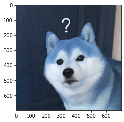
MegEngine uses OpenCV to process images at the bottom layer. Due to historical reasons, OpenCV will store images in BGR order after decoding when the image is 3-channel, and get NumPy ndarray format data ( See document ) . MegEngine follows the processing habits of OpenCV, so in most cases, the default image is BGR order, which needs special attention.

We can choose a picture to decode with OpenCV and Matplotlib respectively, and verify：

>>> image_path = "/path/to/example.jpg"  # Select the same image to read

At this point, if you call plt.imshow (this interface displays pictures in RGB order), you will get inconsistent results：

OpenCV uses BGR order

>>> image = cv2.imread(image_path)
>>> plt.imshow(image)
>>> plt.show()

Matplotlib uses RGB order

>>> image = plt.imread(image_path)
>>> plt.imshow(image)
>>> plt.show()

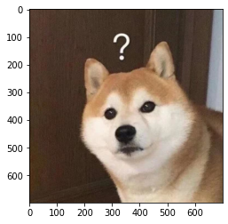
**When reading and writing image data, you need to use the same channel order. ** If you use OpenCV’s cv2.imshow to display the left image, the colors will be displayed normally. And our visualization is using plt.imshow, which displays the image in RGB order, so it needs to be converted.

It is very important to read the instructions on the official website and documentation. The original data on the CIFAR10 homepage is stored in RGB order, while the CIFAR10 interface in MegEngine will have a function that changes the original RGB order to BGR order when processing data. operation to obtain BGR channel sequence data.

Compared with single-channel images, when we do normalization, we need to calculate the corresponding statistics for each channel separately. Here we count：in advance.

>>> mean = [X_train[:,:,:,i].mean() for i in range(3)]
>>> mean
[113.86538318359375, 122.950394140625, 125.306918046875]

>>> std = [X_train[:,:,:,i].std() for i in range(3)]
>>> std
[66.70489964063091, 62.08870764001421, 62.993219278136884]

Consult the ` :class:API documentation and you will find that it accepts the above mean and std as input, for each channel.

Image Tensor layout

In the current CIFAR10 dataset, the shape of each image is $(32, 32, 3)$, also known as HWC layout (Layout) or format (Mode). However, in MegEngine, most of the operators that process 3-channel image Tensor data require the default CHW layout input (no need to understand the reason for now). Therefore, in the last step of preprocessing, we also need to transform the Layout of the image data. Use ToMode interface：

from megengine.data.transform import ToMode

sample = X_train[0]
trans_sample = ToMode().apply(sample)

>>> print(sample.shape, trans_sample.shape)
(32, 32, 3) (3, 32, 32)

Note

Again, the data at this time is still in ndarray format, which is usually converted to Tensor format when it is provided to the model.

See also

• For more transformation operations in the preprocessing stage, please refer to Use Transform to define data transformation ;

• For more introduction to Layout, please refer to the introduction of Tensor memory layout page.

But for the fully connected neural network, whether it is the CHW layout or the HWC layout, the linear layer is used. After flatten, the linear operation will only get neurons in different order, and the final effect will be the same. Yes, next we will see what the shortcomings of fully connected neural networks are.

Think Flatten Handling Again

CIFAR10 数据集 + 全连接神经网络

We use the fully connected neural network in the previous tutorial to train on CIFAR10 (the source code is in examples/beginner/neural-network-cifar10.py ), here we directly use the pre-statistic mean and standard deviation for normalization：

import megengine
import megengine.data as data
import megengine.data.transform as T
import megengine.functional as F
import megengine.module as M
import megengine.optimizer as optim
import megengine.autodiff as autodiff

from os.path import expanduser
DATA_PATH = expanduser("~/data/datasets/CIFAR10")

train_dataset = data.dataset.CIFAR10(DATA_PATH, train=True)
test_dataset = data.dataset.CIFAR10(DATA_PATH, train=False)

train_sampler = data.RandomSampler(train_dataset, batch_size=64)
test_sampler = data.SequentialSampler(test_dataset, batch_size=64)

"""
import nump as np

X_train, y_train = map(np.array, train_dataset[:])
mean = [X_train[:,:,:,i].mean() for i in range(3)]
std = [X_train[:,:,:,i].std() for i in range(3)]
"""

transform = T.Normalize([113.86538318359375, 122.950394140625, 125.306918046875],
                        [66.70489964063091, 62.08870764001421, 62.993219278136884])

train_dataloader = data.DataLoader(train_dataset, train_sampler, transform)
test_dataloader = data.DataLoader(test_dataset, test_sampler, transform)

num_features = train_dataset[0][0].size
num_hidden = 256
num_classes = 10


# Define model
class NN(M.Module):
    def __init__(self):
        super().__init__()
        self.fc = M.Linear(num_features, num_hidden)
        self.classifier = M.Linear(num_hidden, num_classes)

    def forward(self, x):
        x = F.nn.relu(self.fc(x))
        x = self.classifier(x)
        return x


model = NN()

# GradManager and Optimizer setting
gm = autodiff.GradManager().attach(model.parameters())
optimizer = optim.SGD(model.parameters(), lr=0.01)


# Training and validation
nums_epoch = 50
for epoch in range(nums_epoch):
    training_loss = 0
    nums_train_correct, nums_train_example = 0, 0
    nums_val_correct, nums_val_example = 0, 0

    for step, (image, label) in enumerate(train_dataloader):
        image = F.flatten(megengine.Tensor(image), 1)
        label = megengine.Tensor(label)

        with gm:
            score = model(image)
            loss = F.nn.cross_entropy(score, label)
            gm.backward(loss)
            optimizer.step().clear_grad()

        training_loss += loss.item() * len(image)

        pred = F.argmax(score, axis=1)
        nums_train_correct += (pred == label).sum().item()
        nums_train_example += len(image)

    training_acc = nums_train_correct / nums_train_example
    training_loss /= nums_train_example

    for image, label in test_dataloader:
        image = F.flatten(megengine.Tensor(image), 1)
        label = megengine.Tensor(label)
        pred = F.argmax(model(image), axis=1)

        nums_val_correct += (pred == label).sum().item()
        nums_val_example += len(image)

    val_acc = nums_val_correct / nums_val_example

    print(f"Epoch = {epoch}, "
          f"train_loss = {training_loss:.3f}, "
          f"train_acc = {training_acc:.3f}, "
          f"val_acc = {val_acc:.3f}")

The fully connected neural network structure we defined in the previous tutorial can only achieve a classification accuracy of about 50% on CIFAR10, which means it is not qualified. There are also computing modes other than full connections in the neural network model, which can produce different effects when dealing with different types of tasks and data. This requires us to have a deeper understanding and thinking about tasks and data, rather than completely hoping to deepen the network structure and adjust hyperparameters.

Note

• Fully connected neural networks do not work well for higher resolution image data. The larger size of the image will lead to more neurons in the fully connected network, which means that the parameters in the model and the computation amount during training will become huge, and the cost may not be able to Accepted; also, a large number of parameters may cause the model to overfit very quickly during training.

• The input of the fully connected neural network must be a flattened feature vector, so the processing we took before was flatten operation, and did not consider the possible impact. Such an operation can be regarded as a dimensionality reduction of the image data, which will lose a lot of information - such as the local spatial information between each adjacent pixel.

• The fully connected neural network is more sensitive to the change of the pixel position in the image. If the difference between the two pictures is only shifted up and down, the fully connected neural network may think that the spatial information is completely different. Has spatial translation invariance.

Let’s take some inspiration from the traditional field of computer vision, how people exploit the spatial information of images.

digital image processing：filtering

Digital image processing (Digital Image Processing) is a method and technology for removing noise, enhancing, restoring, segmenting, and extracting features through a computer. I won’t cover this area too much in this tutorial, but will focus on filtering and convolution operations in it. First let’s use the ``：interface in OpenCV to have an intuitive understanding.

image_path = "/path/to/example.jpg"  # Select the same image to read
image = plt.imread(image_path)

filters = [np.array([[  0,  0,  0],
                     [  0,  1,  0],
                     [  0,  0,  0]]),
           np.array([[ -1, -2, -1],
                     [  0,  0,  0],
                     [  1,  2,  1]]),
           np.array([[  0, -1,  0],
                     [ -1,  8, -1],
                     [  0, -1,  0]])]

for idx, filter in enumerate(filters):
    result = cv2.filter2D(image, -1, filter)
    plt.subplot(1,3,idx+1)
    plt.axis('off')
    plt.imshow(result)
plt.show()

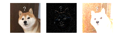
Note： The -1 in cv2.filter2D means to automatically apply the filter matrix to each channel of the picture.

It can be intuitively felt that the filtering operation can process the characteristics of the image well. The steps are：, that is, first fill the original image with 0 value, then calculate the corresponding product of the neighborhood pixel matrix and the filter matrix of each pixel in the image, and then sum it up as the value of the pixel position. As a verification, the pixel is calculated with our first filter matrix above, and the original value is obtained, so the final output is the original image.

In the filtering process, the spatial information of the image is used, and different filters will be used to obtain different effects, such as edge extraction, blurring, sharpening, and so on.

Understanding Convolution Operators

The filtering operation can be understood as a combination of：and Convolution operations.

The above figure is an example to help us better understand the process of convolution calculation. The blue part (bottom) in the figure represents the input channel, the shading on the blue part represents the \(3 \times 3\) convolution kernel (Kernel), and the green part (top) represents the output channel. For each location on the blue input channel, a convolution operation is performed, that is, the shaded part of the blue input channel is mapped to the corresponding shaded part of the green output channel.

In CIFAR10, the input image is 3-channel, so we need to use a kernel of shape \(3 \times 3 \times 3\), a kernel depth of 3 means that there are 3 different filters in the kernel The processor calculates separately with each channel, and the values calculated by different channels at the same position are added together, and finally a 2D output with a shape of \(32 \times 32\) will be obtained (assuming the padding width is 1), which we call features Feature map.

Note

The corresponding Tensor operation interfaces implemented in MegEngine are pad and conv2d (when calling conv2d, you can pass padding" `` parameter to achieve the same effect), the latter is the interface for performing 2D convolution operations on Tensor data in the form of images, and its corresponding :class:`~.module.Module` is :class:`~.module.Conv2d`. In :class:`~.module.Conv2d` There are also：strides (Stride), indicating the distance that the filter moves each time; and there are ``dilation, groups and other parameters, the input needs to be NCHW layout , please refer to the API documentation for specific instructions.

Warning

Strictly speaking, the operation process performed between the input data and the convolution kernel referred to in deep learning is actually a cross-correlation operation, not a convolution operation (the real convolution operation requires The product kernel is flipped diagonally), and we usually do not use the term cross-correlation, which is used to call it convolution.

Let’s see an example of using convolution operation in：

from megengine import Tensor
from megengine.module import Conv2d

sample = X_train[:100]  # NHWC
batch_image = Tensor(sample, dtype="float32").transpose(0, 3, 1, 2)  # NCHW

>>> batch_image.shape
(100, 3, 32, 32)

>>> result = Conv2d(3, 10, (3, 3), stride=1, padding=1)(batch_image)
>>> result.shape
(100, 10, 32, 32)

It can be found that the number of channels has changed from 3 to 10. If you change the settings of the stride and padding parameters, the height and width of the output feature map will also change, which is different from the filtering operation. . Compared with the fully connected layer, each neuron in the convolutional layer only pays attention to the part of interest when calculating, and can make better use of the spatial information of the image. The convolution operation can be understood as a feature extraction operation, which can learn information from the image <https://cs231n.github.io/understanding-cnn/>`_ .

Convolutional Neural Network Architecture Patterns

The most popular convolutional neural network architecture patterns are:

[Conv->Actication->Pooling]->flatten->[Linear->Actication]->Score.

• In the neural network, if you want to introduce nonlinearity into the model, you need to add an activation function after the calculation is completed, and the same is true for the convolutional layer;

• In addition, after the feature extraction is completed using the convolutional layer, a pooling (Pooling) operation such as MaxPool2d is usually used. The logic is to perform downsampling operations along the spatial dimension (height, width), that is, only a piece of local information is retained in an area as a representative. One explanation is that such an operation enables the convolutional neural network model to have better generalization capabilities; it gradually reduces the size of the image space to reduce the amount of parameters and computation in the network, thereby controlling overfitting .

• When enough raw features are extracted using convolutional layers, fully connected layers can be used for classification like MNIST data.

The introduction here is a bit brief. For a more detailed explanation, please refer to the Official Note of the Stanford CS231n course.

Practice：Convolutional Neural Networks

The next thing we have to do is “see pictures and talk”, implement a convolutional neural network and classify：

We refer to the LeNet [2] network, and the structure of its model is shown in the figure below (the picture is taken from the paper)：

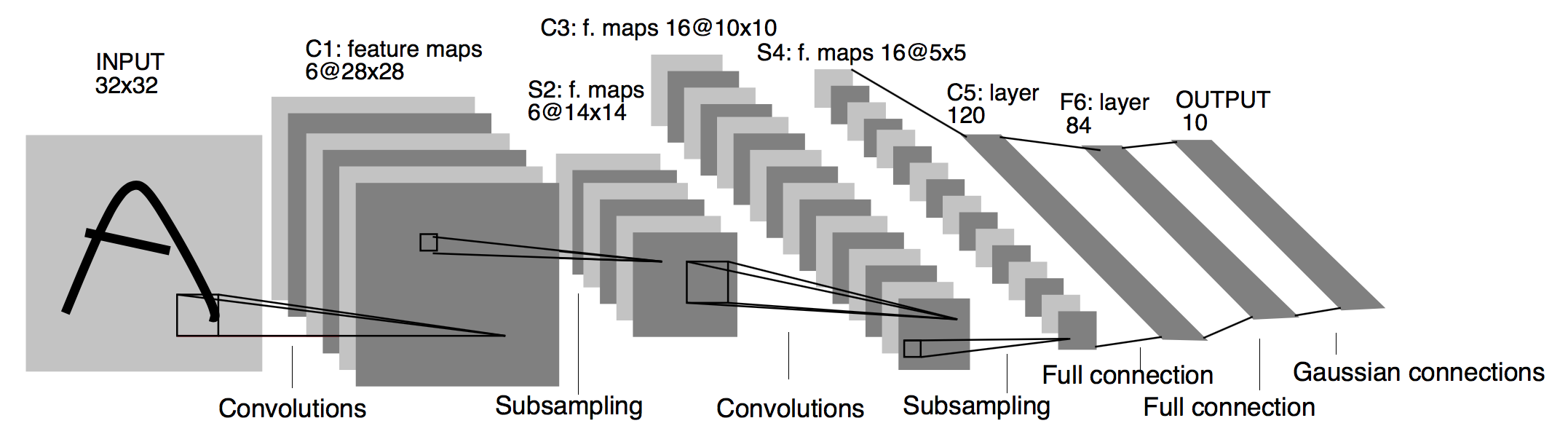
Architecture of LeNet a Convolutional Neural Network here for digits recognition. Each plane is a feature map ie a set of units whose weights are constrained to be identical.

Note：that we used Compose in data preprocessing to compose the various transformations.

import megengine
import megengine.data as data
import megengine.data.transform as T
import megengine.functional as F
import megengine.module as M
import megengine.optimizer as optim
import megengine.autodiff as autodiff


from os.path import expanduser
DATA_PATH = expanduser("~/data/datasets/CIFAR10")

train_dataset = data.dataset.CIFAR10(DATA_PATH, train=True)
test_dataset = data.dataset.CIFAR10(DATA_PATH, train=False)

train_sampler = data.RandomSampler(train_dataset, batch_size=64)
test_sampler = data.SequentialSampler(test_dataset, batch_size=64)

"""
import nump as np

X_train, y_train = map(np.array, train_dataset[:])
mean = [X_train[:,:,:,i].mean() for i in range(3)]
std = [X_train[:,:,:,i].std() for i in range(3)]
"""

transform = T.Compose([
    T.Normalize([113.86538318359375, 122.950394140625, 125.306918046875],
                [66.70489964063091, 62.08870764001421, 62.993219278136884]),
    T.ToMode("CHW"),
])

train_dataloader = data.DataLoader(train_dataset, train_sampler, transform)
test_dataloader = data.DataLoader(test_dataset, test_sampler, transform)


# Define model
class ConvNet(M.Module):
    def __init__(self):
        super().__init__()
        self.conv1 = M.Conv2d(3, 6, 5)
        self.conv2 = M.Conv2d(6, 16, 5)
        self.fc1 = M.Linear(16*5*5, 120)
        self.fc2 = M.Linear(120, 84)
        self.classifier = M.Linear(84, 10)

        self.relu = M.ReLU()
        self.pool = M.MaxPool2d(2, 2)

    def forward(self, x):
        x = self.pool(self.relu(self.conv1(x)))
        x = self.pool(self.relu(self.conv2(x)))
        x = F.flatten(x, 1)
        x = self.relu(self.fc1(x))
        x = self.relu(self.fc2(x))
        x = self.classifier(x)
        return x


model = ConvNet()

# GradManager and Optimizer setting
gm = autodiff.GradManager().attach(model.parameters())
optimizer = optim.SGD(model.parameters(), lr=0.01)


# Training and validation
nums_epoch = 50
for epoch in range(nums_epoch):
    training_loss = 0
    nums_train_correct, nums_train_example = 0, 0
    nums_val_correct, nums_val_example = 0, 0

    for step, (image, label) in enumerate(train_dataloader):
        image = megengine.Tensor(image)
        label = megengine.Tensor(label)

        with gm:
            score = model(image)
            loss = F.nn.cross_entropy(score, label)
            gm.backward(loss)
            optimizer.step().clear_grad()

        training_loss += loss.item() * len(image)

        pred = F.argmax(score, axis=1)
        nums_train_correct += (pred == label).sum().item()
        nums_train_example += len(image)

    training_acc = nums_train_correct / nums_train_example
    training_loss /= nums_train_example

    for image, label in test_dataloader:
        image = megengine.Tensor(image)
        label = megengine.Tensor(label)
        pred = F.argmax(model(image), axis=1)

        nums_val_correct += (pred == label).sum().item()
        nums_val_example += len(image)

    val_acc = nums_val_correct / nums_val_example

    print(f"Epoch = {epoch}, "
          f"train_loss = {training_loss:.3f}, "
          f"train_acc = {training_acc:.3f}, "
          f"val_acc = {val_acc:.3f}")

After nearly 50 rounds of training, a LeNet model with an accuracy rate of more than 60% can usually be obtained, which is better than simply using a fully connected neural network.

In this tutorial, you were introduced to the basic concepts of Convolutional Neural Networks and were trained and evaluated on the CIFAR10 dataset using the LeNet model. In fact, the LeNet model can achieve over 99% classification accuracy on the MNIST dataset, which is also the example we gave in “Getting started with MegEngine”, you should be able to fully understand this tutorial by now.

See also

The corresponding source code for this tutorial： examples/beginner/linear-classification.py

Summary：Alchemy is not entirely metaphysical

In the field of deep learning, the model is the alchemy formula, the data is the spiritual material, the GPU device is the real fire of samadhi, and the MegEngine is a powerful alchemy furnace.

As an alchemist, it may indeed take a lot of time in the “parameter adjustment” step, and some metaphysical phenomena will always occur. But after this series of tutorials, I believe you have also recognized some deeper content, let us review the concept of machine learning again：

A computer program is said to learn from experience E with respect to some class of tasks T and performance measure P, if its performance at tasks in T, as measured by P, improves with experience E.

A computer program is said to have learned from experience E if it can improve its performance P on some class of tasks T based on experience E.

In guiding machines to learn, we need a deeper understanding of experience,：, and performance.

• Experience：Model experience in deep learning usually comes from datasets and losses (learning from mistakes). In this tutorial, there is not much knowledge about data standardization and preprocessing. However, in practical engineering practice, the quality of data is also very critical, and more data usually brings better performance. It is also important to design a scientific loss function, which directly determines our optimization goals.

• Task：Many times, knowledge in traditional fields will bring us a lot of other things, and machines can do some tasks more efficiently than humans;

• Performance：We use evaluation metrics for different tasks, and this series of tutorials is just the tip of the iceberg.

Expansion material

模型保存与加载

Although GPU devices can achieve dozens of times or even better acceleration than CPUs, you may have found some problems. The time will be longer and longer, how to count the amount of parameters and calculations, and how to save and load our model? Please find a solution by consulting the MegEngine documentation, and implement it.

经典 CNN 模型结构

We haven’t touched some classic convolutional neural network architectures like AlexNet, GoogLeNet, VGGNet, ResNet, etc. Reproducing these models is a great form of exercise, and it is recommended that you scour the material for this challenge yourself. In addition, in the BaseCls code base of Megvii Science and Technology Research Institute, we can find a lot of pre-training models based on MegEngine, and you can do many things with pre-training models. These contents are also essential skills on the way to become an alchemist, and we will introduce them in more detail in the next tutorial.

references

[1]

Alex Krizhevsky, Vinod Nair, and Geoffrey Hinton. Cifar-10 (canadian institute for advanced research). URL: http://www.cs.toronto.edu/~kriz/cifar.html.

[2]

Yann LeCun, Léon Bottou, Yoshua Bengio, and Patrick Haffner. Gradient-based learning applied to document recognition. Proceedings of the IEEE, 86(11):2278–2324, 1998.