MegEngine implements linear classification#
What this tutorial covers
Have a basic understanding of image coding in the field of computer vision and understand the classification tasks in machine learning;
Think about what changes the linear regression model has undergone to solve the classification task, and what evaluation metrics should be used;
According to the previous introduction, use MegEngine to implement a linear classifier to complete the MNIST handwritten digit classification task.
Visual operation
There is some data visualization in this tutorial, if you have no experience with Matplotlib, just focus on the output.
Get the original dataset#
In the previous tutorial, we used the interface in Scikit-learn to get California housing data, and mentioned that many Python libraries and frameworks will encapsulate the interface to get some datasets, which is convenient for users to call. MegEngine is no exception. In data.dataset module, you can get Use the implemented data set interface to get the original data set, such as MNIST data set used in this tutorial.
from megengine.data.dataset import MNIST
from os.path import expanduser

DATA_PATH = expanduser("~/data/datasets/MNIST")

train_dataset = MNIST(DATA_PATH, train=True)
test_dataset = MNIST(DATA_PATH, train=False)
Different from the data format obtained in the previous tutorial, what is obtained here is the already divided training set train_dataset and test set test_dataset, and both have been encapsulated into MegEngine and can be provided to Dataset type of DataLoader` (for details, please refer to Use Dataset to define a data set). where each element is a tuple \((X_i, y_i)\) :consisting of a single sample \(X_i\) and a token \(y_i\)
>>> type(train_dataset[0])
tuple
In order to facilitate the following discussion, we deliberately split the samples and labels of the training data into:
import numpy as np

X_train, y_train = map(np.array, train_dataset[:])
>>> print(X_train.shape, y_train.shape)
(60000, 28, 28, 1) (60000,)
Statistical mean and standard deviation information of training samples, normalized to:for data preprocessing
>>> mean, std = X_train.mean(), X_train.std()
>>> print(mean, std)
33.318421449829934 78.56748998339798
Note
For classic datasets such as MNIST, these statistics are usually provided on the dataset homepage, or you can find data that others have already calculated on the Internet with the help of search engines.
Learn about dataset information#
Recall that in the last tutorial, our housing sample data (before splitting) has a shape of \((20640, 8)\), which means that there are 20640 samples in total, each with 8 attribute values. It can also be said that is the dimension of the feature vector is 8. And the shape of the training data here is \((60000, 28, 28, 1)\), if 60000 is the total number of training samples, then the following \((28, 28, 1)\) shape What does it stand for?
MNIST 数据集
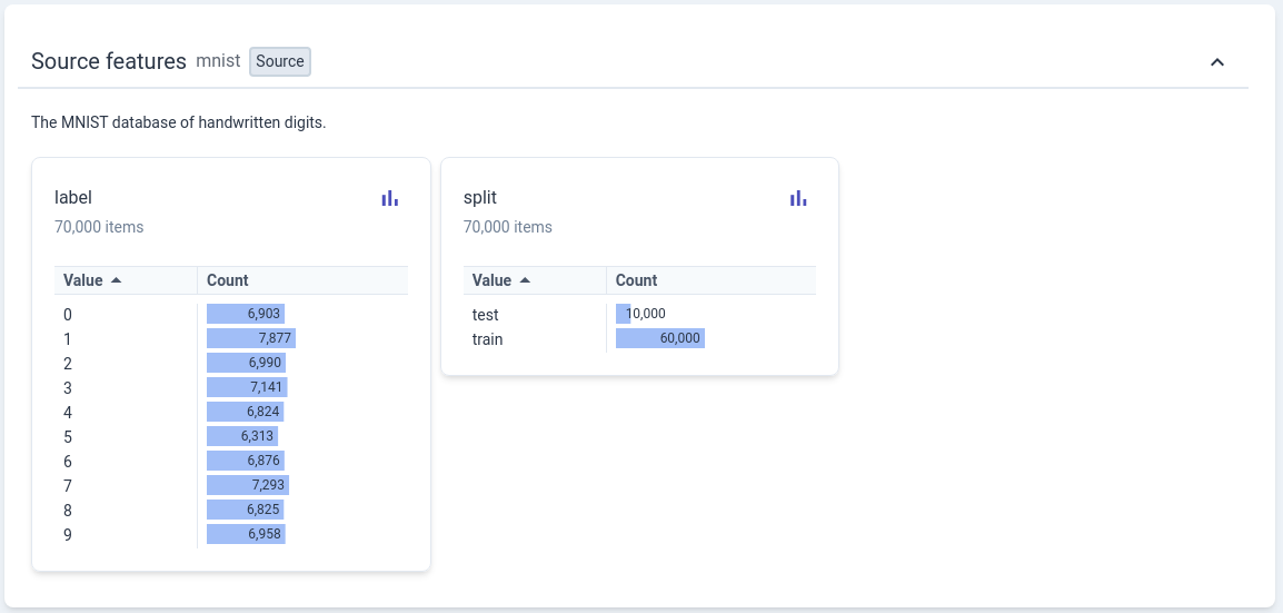
Query the MNIST official website homepage [1] for the introduction information.: The handwritten digits dataset contains 60,000 training images and 10,000 testing images, each image is a grayscale image of 28x28 pixels. Google provides a website called Know Your Data that can help us understand some classic public datasets in a visual way, including the MNIST dataset used here.
Marker \(y \in \left\{ 0, 1, \ldots , 9 \right\}\) is a discrete numerical value, not the same as the sample marker value (house price) \(y \in \mathbb R\) in the previous tutorial Same.#
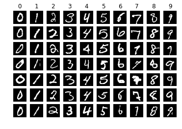
Running the following visualization code can help you have an intuitive understanding of the data (no need to understand the code implementation at present):
import matplotlib.pyplot as plt

classes = ['0', '1', '2', '3', '4', '5', '6', '7', '8', '9']
num_classes = len(classes)
samples_per_class = 7

for y, cls in enumerate(classes):
    idxs = np.squeeze(np.where(y_train == y))
    idxs = np.random.choice(idxs, samples_per_class, replace=False)
    for i, idx in enumerate(idxs):
        plt_idx = i * num_classes + y + 1
        plt.subplot(samples_per_class, num_classes, plt_idx)
        plt.imshow(X_train[idx].squeeze(), cmap="gray")
        plt.axis('off')
        if i == 0:
            plt.title(cls)
plt.show()
验证集(开发集)藏在哪里
In many publicly available datasets, dataset providers have divided training and test sets for users. But as we mentioned in the last tutorial, we should at least also provide a validation set to avoid overfitting on the training set. In actual practice, there will be many strange divisions of such data sets. Take our existing:training set and test set as an example.
If we further divide the 60000 samples in the training set into training set and validation set according to the ratio of 5:1. This way of handling is the same as in the previous tutorial, at this time the test set is responsible for simulating the “unpredictable” data in the future production environment, and it is only used once;
If we further divide the 10,000 samples in the current test set into a validation set and a test set in a ratio of 1:1, there are different implications. The starting point of this approach is that the “validation: ” should be a simulation of the “test set” and should try to maintain the same distribution as the test set. For example, in the machine learning competition, the test set \(T_a\) provided to the players may be a part of the original test set \(T\), and the ranking in the public list is given on the \(T_a\) score, and the final ranking will be done on the real test set \(T_b\).
If we do not further divide the training set and the test set here, but verify on the existing test set after each round of training, it means that the test set actually plays the role of the verification set. So where is the real test set? It comes from our production environment. After all, the definition of the test set is “unpredictable” data, and it is often impossible to obtain it in advance.
All in all, the division strategy of the data set depends more on what kind of data we can obtain and whether it is consistent with the data distribution in future usage scenarios. The terms test set and validation set are often used interchangeably (or refer to each other), so the easiest way to judge is by purpose. What needs to be:is that in the process of model training, timely verification of model performance is an indispensable process.
In this tutorial, the MNIST test set is treated as the validation set, that is, after each round of parameter update, the performance of the model on the test set will be evaluated.
Unstructured data:pictures#
In the California housing dataset, we can use the feature vector \(\mathrm{x} \in \mathbb{R}^d\) to describe the characteristics of housing. The entire data set can be expressed and stored with the help of a two-dimensional table (matrix). We call such data structured data. In real life, it is easier for humans to touch and understand unstructured data, such as video, audio, pictures, etc…
How do computers understand, represent, and store such data? This tutorial will illustrate the example of a sample handwritten digit picture in:
>>> idx = 28204
>>> plt.title("The label is: %s" % y_train[idx])
>>> plt.imshow(X_train[idx].squeeze(), cmap="gray")
>>> plt.show()
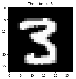
The images in the MNIST dataset are all bitmap images (Bitmap), also called raster images, raster images, as opposed to the concept of vector graphics; each image consists of many points called pixels (Pixel, Pictrue element) composition. We take a picture sample marked 3 X_train[idx] for observation, and find that its height (Height) and width (Weight) are both 28 pixels, which is similar to the shape of a single sample :math:`(28, 28, 1) ` Corresponding; the last dimension represents the number of channels. Since the image in MNIST is a grayscale image, the number of channels is 1. For color images in the RGB color system, the number of channels is 3, which we will cover in the next tutorial. see data like this.
Now let’s visualize this grayscale image in 3 dimensions to help develop an intuitive understanding of:
>>> from mpl_toolkits.mplot3d import Axes3D
>>> ax = plt.axes(projection='3d')
>>> ax.set_zlim(-10, 255)
>>> ax.view_init(elev=45, azim=10)
>>> X, Y = np.meshgrid(np.arange(28), np.arange(28))
>>> Z = np.squeeze(X_train[idx])
>>> surf = ax.plot_surface(Y, X, Z, cmap="gray")
>>> plt.colorbar(surf, shrink=0.5, aspect=8)
>>> plt.show()
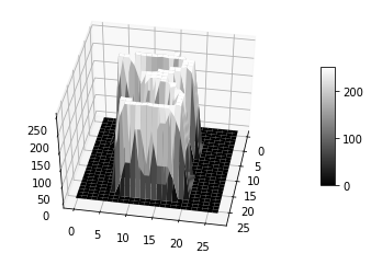
In a grayscale image, each pixel value is represented by 0 (black) ~ 255 (white), which is the range that an int8 can represent.
We usually call \((60000, 28, 28, 1)\) such data as NHWC layout, we will see more layout forms later.
Simple processing of image features#
Differences in features between different types of data
In the previous tutorial, the one-shot input to the linear model was a feature vector \(\mathrm{x} \in \mathbb{R}^d\);
And the feature space of picture \(\mathsf{I}\) in the MNSIT dataset here is \(\mathbb{R}^{H \times W \times C}\).
In order to meet the requirements of the linear model for the input shape, it is necessary to perform certain processing on the characteristics of the input samples. The easiest and crudest way to implement \(\mathbb{R}^{H \times W \times C} \mapsto \mathbb{R}^d\) without losing the numerical information of each element is to use the flatten flattening operation:
The original image
original_image = np.linspace(0, 256, 9).reshape((3, 3))
plt.axis('off')
plt.title(f"Original Image {original_image.shape}:")
plt.imshow(original_image, cmap="gray")
plt.show()

After Flatten processing
flattened_image = original_image.flatten()
plt.axis('off')
plt.title(f"Flattened Image {flattened_image.shape}:")
plt.imshow(np.expand_dims(flattened_image, 0), cmap="gray")
plt.show()

The corresponding interface in MegEngine is Tensor.flatten or functional.flatten. Same as expand_dims and squeeze operations mentioned in the previous tutorial, :func:` The ~.flatten` operation can also be implemented with reshape. But considering the code semantics, you should try to use flatten instead of reshape.
The flattening operation in MegEngine can be directly used in the case of multiple samples (in order to support vectorized calculations):
import megengine.functional as F

x = F.ones((10, 28, 28, 1))
out = F.flatten(x, start_axis=1, end_axis=-1)
>>> print(x.shape, out.shape)
(10, 28, 28, 1) (10, 784)
After a simple process, it is possible to correlate the single-sample linear prediction model with the form \(\hat{y} = \boldsymbol{w} \cdot \boldsymbol{x}+b\) from the previous tutorial.
The output form of the classification task#
In a linear regression task, our predicted output value \(\hat{y}\) is continuous on the real number domain \(\mathbb R\). For classification tasks, the labels are usually given as a set of discrete values, such as \(y \in \left\{ 0, 1, \ldots , 9 \right\}\) here. What about achieving unity of model prediction output and labeling form?
Let’s simplify the problem form first, starting with the simplest classification case, the binary classification task.
binary classification task#
Suppose our handwritten digit classification task is simplified to the case where the tokens only contain 0 and 1, ie \(y \in \left\{ 0, 1 \right\}\). Where 0 means that the picture is a handwritten digit 0, and 1 means that the image is not a handwritten number 0. For discrete tokens, we can introduce a non-linear link function \(g(\cdot)\) to map the linear output to categories. For example, you can divide the output of \(f(\boldsymbol{x})=\boldsymbol{x} \cdot \boldsymbol{w}+b\) with 0 as the threshold (Threshold), and think that any sample whose calculation result is greater than 0 represents this picture is the handwritten number 0; and any sample whose calculation result is less than 0 means that the picture is not a handwritten number 0. Therefore, such a prediction model can be:
Where \(\mathbb I\) is the indicator function (also called the indicative function), which is also the link function we use here, but it is not commonly used. There are many reasons, for optimization problems, its mathematical properties are not good and it is not suitable for gradient descent algorithm. For the outputs of the linear model -100 and -1000, this piecewise function decides both to be in the class marked 0, and does not reflect the difference within the two sample classes - for example, although both are Not 0, but a sample with an output of -1000 should be less like 0 than a sample with an output of -100. The former might be 1, the latter 6.
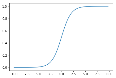
In practice, the link function we use more often is the Sigmoid function \(\sigma(\cdot)\) (also called the Logistic function):
def sigmoid(x):
    return 1. / (1. + np.exp(-x))

x = np.arange(-10, 10, 0.2)
y = sigmoid(x)
plt.plot(x, y)
plt.show()
where \(\exp\) refers to the exponential function:with the natural constant \(e\) as the base
Sigmoid / Logistic 命名的由来,与 Logit 函数
Logistic was named by Belgian mathematician Pierre François Verhulst in 1844 or 1845 when he was studying the relationship between population growth. Like Sigmoid, it refers to the sigmoid function:The initial stage is roughly exponential growth; then as it begins to become saturated, the increase slows down Finally, the increase stops when maturity is reached. Here’s Verhulst’s explanation of the naming:
Verhulst writes “We will give the name logistic [logistique] to the curve” (1845 p.8). Though he does not explain this choice, there is a connection with the logarithmic basis of the function. Logarithm was coined by John Napier (1550- 1617) from Greek logos (ratio, proportion, reckoning) and arithmos (number). Logistic comes from the Greek logistikos (computational). In the 1700’s, logarithmic and logistic were synonymous. Since computation is needed to predict the supplies an army requires, logistics has come to be also used for the movement and supply of troops.
Berkson coined logit (pronouced “low-jit”) in 1944 as a contraction of logistic unit to indicate the unit of measurement (J. Amer. Stat. Soc. 39:357-365). Georg Rasch derives logit as a contraction of logistic transform (1980, p.80). Ben Wright derives logit as a contraction of log-odds unit. Logit is also used to characterize the logistic function in the way that probit (probability unit, coined by Chester Bliss about 1934), characterizes the cumulative normal function.
The inverse function of Sigmoid is the Logit function, that is, \(\text{logit}(p) = \log(\frac{p}{1-p})\), there are \(\sigma (\text{logit}(p))=p\). According to Sigmoid, real numbers can be Properties that map to probabilities, it’s easy to see that Logit is able to map probabilities to real numbers.
Another reason to choose Sigmoid is that it has a good mathematical explanation from an information theory perspective (not covered in detail in this tutorial), which can be derived under the assumptions of Bernoulli distribution and generalized linear models according to the principle of Maximum entroy . Models that use Sigmoid / Logistic functions are also called Logistic Regression Models (LR Models). It is translated as “logistic regression” in many places, which is as confusing as the translation of Robustness into “robustness”, which is more suitable for translation as logarithmic probability regression in terms of mathematical properties.
This logistic term will not be translated in this tutorial.
We found that for binary classification tasks, the sigmoid function has the following advantages:
Easy to differentiate:\(\sigma^{\prime}(x)=\sigma(x)(1-\sigma(x))\)
The output of the linear calculation part is mapped to the range of \((0, 1)\) and can be expressed as a probability.
We can express the probability of predicting the label of sample \(\mathrm{x}\) to be a certain class (assuming 1 here):
Continue to use the example:we gave above for the output of the linear model, after the mapping of the Sigmoid function, \(\sigma(-1000)\) is closer to 0 than \(\sigma(-100)\), indicating that the former is not 0 probability is higher. This enables the difference between the prediction results of different samples to be effectively reflected. At the same time, for samples that have been correctly classified, the sigmoid function discourages stretching the output range of the linear model too large, and the benefit is not obvious.
Warning
The final output of binary logistic regression has only one value, which represents the probability of predicting a base class. Next we will introduce Multiclass Logistic Regression (Multinational Logistic Regression).
Multi-classification tasks#
Converting the output of a classification model to a probabilistic representation of the target class is a very common (but not unique) approach. The final output in logistic regression has only one probability \(p\), which represents the probability of predicting a certain category; the probability of another category can be directly represented by \(1-p\). Generalizing to multi-classification tasks, how do we transform the output of a linear model into probabilistic predictions over multiple classes?
One-hot encoding of markers
Astute readers may have noticed this, the tokens in the MNIST dataset are all scalars. Therefore, some additional processing is required to turn it into a probability vector on multi-classification. The common practice is to use One-hot encoding. For example, the corresponding marks of two handwritten digit samples are 3 and 5, using One-hot encoding (the corresponding interface is functional.nn.one_hot ) will get the following representation:
from megengine import Tensor
import megengine.functional as F

inp = Tensor([3, 5])  # two labels
out = F.nn.one_hot(inp, num_classes=10)
>>> out.numpy()
array([[0, 0, 0, 1, 0, 0, 0, 0, 0, 0],
       [0, 0, 0, 0, 0, 1, 0, 0, 0, 0]], dtype=int32)
After this processing, the label of each sample becomes a 10-class probability vector that can be compared with the model prediction output.
Recalling the form of linear regression, for a single sample \(\boldsymbol x \in \mathbb{R}^d\), with the help of the weight vector \(\boldsymbol{w} \in \mathbb{R}^d\) and the bias \(b\), you can Get a linear output \(\boldsymbol {w} \cdot \boldsymbol {x} + b\), now we can think of this output as the score \(s\) predicting that the current sample is a certain category, or predicting the credibility of the category Spend. For \(c\) classification tasks, we want to get \(c\) such scores, so we can achieve:with the help of matrix operations
Note that:is written here in the form of matrix operations in linear algebra for ease of understanding. In actual calculations, it is not necessary to upgrade vectors to matrices.
Let’s simply verify that the output score is a 10-dimensional vector (using the matrix@vector operation in the previous tutorial):
num_features = 784  # Flatten(28, 28, 1)
num_classes = 10

x = X_train[0].flatten()
W = np.zeros((num_classes, num_features))
b = np.zeros((num_classes,))
s = W @ x + b
>>> s.shape
(10,)
We can intuitively understand that a \(d\) dimensional feature vector can get a \(c\) dimensional score vector after a weight matrix transformation and bias.
The sigmoid function is able to map a single output from the real number domain \(\mathbb R\) to the probability interval \((0,1)\) , for a score vector. If you apply the sigmoid function for each class score, you do get multiple probability values, but the problem is that the probability values obtained in this way do not sum to 1. Need to find other ways.
The easiest way to think of it is to learn the One-hot representation, set the probability at the maximum value (corresponding to interface functional.argmax) to 1, and all other positions to 0. For example, \((10, -10, 30 , 20)\) becomes \((0, 0, 1, 0)\). \(\operatorname{Argmax}\) This approach belongs to hard classification, and the indicative function :math:seen earlier in the binary classification task mathbb I (cdot ) has the same problem:that the mathematical properties are relatively poor; the difference between samples within a class, between classes cannot be reflected… and so on.
In multi-classification tasks, the more commonly used function is \(\operatorname{Softmax}\) (corresponding to interface functional.nn.softmax ):
It can be understood that we get the target classification probability value after exponential normalization of the scores on multiple classes, which we usually call Logits;
This exponential form of normalization has some advantages:compared to the mean normalization, it has a “Matthew effect”, we think that the larger original value should also have a larger probability value after normalization; Compared with hard classification \(\operatorname{Argmax}\), it is softer, which can reflect the difference between the predicted values of samples within and between classes; it is beneficial to find the Top-k classification candidates, that is, the first \(k\) have high probability Classification, useful for evaluating model performance.
>>> score = Tensor([1, 2, 3, 4])
>>> F.softmax(score)
Tensor([0.0321 0.0871 0.2369 0.6439], device=xpux:0)
At this point, we’ve been able to get our model to output a probability vector of predictions on the target class based on the input samples.
Optimization Objectives for Classification Tasks#
We have obtained the probability vector \(\hat{\boldsymbol{y}}\) predicted by the model on multi-classification, and also obtained the probability vector \(\boldsymbol{y}\) by using One-hot encoding for the real mark. a probability distribution. Our optimization goal is to make the predicted values as close as possible to the ground truth, and we need to design a suitable loss function.
Relative Entropy and Cross Entropy in Information Theory
In information theory, if there are two separate probability distributions \(p(x)\) and \(q(x)\) for the same random variable \(x\), the relative entropy (KL divergence) can be used to represent the two Difference Between Distributions:
The characteristic of relative entropy is that when two probability distributions are exactly the same, its value is zero. The greater the difference between the two distributions, the greater the relative entropy value.
This coincides with our goal of “designing a loss function that can be used to evaluate the difference between the probability distribution \(q(x)\) of the current prediction and the probability distribution \(p(x)\) of the true labels”. And since the sample label will not change during the training process, its probability distribution \(p(x)\) is a definite constant, then the \(H(p)\) value in the above formula will not change with the change of the training sample, It will not affect the gradient calculation, so it can be omitted.
The remaining \(H(p, q)\) part is defined as our commonly used cross entropy (Cross Entropy, CE), which is:in terms of discrete probability values in our current example
This is the loss function often used in classification tasks, corresponding to the functional.nn.cross_entropy interface in MegEngine.
使用 cross_entropy 接口时的注意事项
The cross_entropy interface in MegEngine is designed with the actual usage scenario in:
One-hot encoding is performed on the tag value by default, which does not require the user to manually process it in advance;
By default, the Softmax calculation is first converted into a class probability value (ie
with_logits=True).
Therefore, when writing model code, you will find that one_hot and softmax interfaces do not need to be used.
As a demonstration, the following shows three cases where the predicted value and the actual value are calculated to obtain the cross:loss.
label = Tensor(3)
pred_list = [Tensor([0., 0., 0., 1., 0.,
                     0., 0., 0., 0., 0.]),
             Tensor([0., 0., 0.3, 0.7, 0.,
                     0., 0., 0., 0., 0.]),
             Tensor([0., 0., 0.7, 0.3, 0.,
                     0., 0., 0., 0., 0.])]
for pred in pred_list:
    print(F.nn.cross_entropy(F.expand_dims(pred, 0),
                             F.expand_dims(label, 0),
                             with_logits=False).item())
0.0
0.3566749691963196
1.2039728164672852
Evaluation Metrics for Classification Tasks#
Commonly used evaluation metrics in regression problems are MAE, MSE, etc., but they are not suitable for classification tasks.
In this tutorial, we will introduce Accuracy as an evaluation metric for handwritten digit image classification. Its definition is as follows::is the proportion of correctly classified samples to all samples. For example, out of 10,000 samples, if 6,000 samples are correctly classified, then we say that the accuracy of the current classifier is 0.6, which is 60% when converted into a percentage.
For the multiple outputs on the multi-class predicted by the model, we usually use the argmax interface to use the 0 ~.argmax interface to take the label corresponding to the largest position as the predicted classification, and compare it with the real label (if it is a vectorized implementation of batch samples , usually need to specify the axis parameter):
logits = Tensor([0., 0., 0.3, 0.7, 0.,
                 0., 0., 0., 0., 0.])
pred = F.argmax(logits)
>>> pred
Tensor(3, dtype=int32, device=xpux:0)
For the output obtained on multiple samples, we can use the == operation to judge, taking the prediction results on 5 samples as an example:
>>> pred = Tensor([0, 3, 2, 4, 5])
>>> label = Tensor([0, 3, 3, 5, 2])
>>> pred == label
Tensor([ True  True False False False], dtype=bool, device=xpux:0)
At this time, with the help of sum interface, you can get the number of correctly classified samples:
>>> (pred == label).sum().item()
2
In the process of training the linear classifier, after each round of training, the classification accuracy of the current classifier on the training samples and test samples can be detected as a means of evaluating the model performance. If after many rounds of training, the accuracy on the training set keeps rising and the accuracy on the test set starts to drop, it may be an indication of overfitting.
See also
Accuracy is not the only evaluation metric for classification tasks, and we will touch on more evaluation metrics in later tutorials.
MegEngine also provides
topk_accuracyto calculate Top-k accuracy, but in this tutorial, in order to demonstrate the calculation process (corresponding to the case ofk=1), this interface is not used directly.
Exercise:Linear Classifier#
Combining all the concepts mentioned above, now we use:for a complete implementation of the linear classifier.
You can change the code of the corresponding link according to the process of the previous tutorial, and experience the whole logic;
Note again that in this tutorial the test set provided by MNIST is used as the validation set (albeit named
test);For batches of data, remember to use a vectorized implementation instead of a for loop implementation on a single sample.
import megengine
import megengine.data as data
import megengine.data.transform as T
import megengine.functional as F
import megengine.optimizer as optim
import megengine.autodiff as autodiff


# Get train and test dataset and prepare dataloader
from os.path import expanduser
DATA_PATH = expanduser("~/data/datasets/MNIST")

train_dataset = data.dataset.MNIST(DATA_PATH, train=True)
test_dataset = data.dataset.MNIST(DATA_PATH, train=False)

train_sampler = data.RandomSampler(train_dataset, batch_size=64)
test_sampler = data.SequentialSampler(test_dataset, batch_size=64)

transform = T.Normalize(33.318421449829934, 78.56748998339798)

train_dataloader = data.DataLoader(train_dataset, train_sampler, transform)
test_dataloader = data.DataLoader(test_dataset, test_sampler, transform)

num_features = train_dataset[0][0].size
num_classes = 10


# Parameter initialization
W = megengine.Parameter(F.zeros((num_features, num_classes)))
b = megengine.Parameter(F.zeros((num_classes,)))


# Define linear classification model
def linear_cls(X):
    return F.matmul(X, W) + b


# GradManager and Optimizer setting
gm = autodiff.GradManager().attach([W, b])
optimizer = optim.SGD([W, b], lr=0.01)


# Training and validation
nums_epoch = 5
for epoch in range(nums_epoch):
    training_loss = 0
    nums_train_correct, nums_train_example = 0, 0
    nums_val_correct, nums_val_example = 0, 0

    for step, (image, label) in enumerate(train_dataloader):
        image = F.flatten(megengine.Tensor(image), 1)
        label = megengine.Tensor(label)

        with gm:
            score = linear_cls(image)
            loss = F.nn.cross_entropy(score, label)
            gm.backward(loss)
            optimizer.step().clear_grad()

        training_loss += loss.item() * len(image)

        pred = F.argmax(score, axis=1)
        nums_train_correct += (pred == label).sum().item()
        nums_train_example += len(image)

    training_acc = nums_train_correct / nums_train_example
    training_loss /= nums_train_example

    for image, label in test_dataloader:
        image = F.flatten(megengine.Tensor(image), 1)
        label = megengine.Tensor(label)
        pred = F.argmax(linear_cls(image), axis=1)

        nums_val_correct += (pred == label).sum().item()
        nums_val_example += len(image)

    val_acc = nums_val_correct / nums_val_example

    print(f"Epoch = {epoch}, "
          f"train_loss = {training_loss:.3f}, "
          f"train_acc = {training_acc:.3f}, "
          f"val_acc = {val_acc:.3f}")
After 5 rounds of training, a linear classifier with an accuracy rate of about 92% is usually obtained.
See also
The corresponding source code for this tutorial: examples/beginner/linear-classification.py
Summarize the flow of:data#
So far, we’ve done line fitting, house price prediction, and handwritten digit recognition tasks with linear models, so it’s time for a comparison.
task name |
Forward computation (single sample) |
loss function |
Evaluation Metrics |
|---|---|---|---|
Fit straight line |
\(x \in \mathbb{R} \stackrel{w,b}{\mapsto} y \in \mathbb{R}\) |
MSE |
observed fit |
house price forecast |
\(\boldsymbol{x} \in \mathbb{R}^{d} \stackrel{\boldsymbol{w},b}{\mapsto} y \in \mathbb{R}\) |
MSE |
MAE |
Handwritten Digit Recognition |
\(\boldsymbol{x} \in \mathbb{R}^{d} \stackrel{W,\boldsymbol{b}}{\mapsto} \boldsymbol{y} \in \mathbb{R}^{c}\) |
CE |
Accuracy |
Note:The default image information has been flattened into a vector, ie :math:`mathsf{I} in mathbb{R}^{H times W times C} stackrel{operatorname{flatten}}{mapsto} boldsymbol{x} in mathbb{R}^{d}
When implementing with MegEngine, we need to pay attention to the flow of single sample data in the entire calculation graph, especially the change of Tensor shape (essentially these are common transformations in linear algebra), which is actually our machine learning model In the design process, in addition to the linear model itself, the entire machine learning process also needs to design an appropriate loss function and select scientific evaluation indicators.
In other respects, the practices of several tasks are the same. For example, for batch-sized data, the vectorized implementation is used to speed up, and the gradient descent algorithm is used to iteratively optimize the parameters in the model, and it is necessary to evaluate the model performance in time. …hopefully you already have a better understanding of these steps.
It seems that linear models can do everything?
the answer is negative. Since the datasets in these tutorials are too simple, even using the simplest linear model for training can achieve relatively good results in the end. In the next tutorial, we will use a more complex dataset (compared to MNIST only slightly more complex), the same classification task, to see if the linear model is still as powerful.
Expansion material#
尝试使用其它的机器学习算法完成分类任务
Please try to understand the K nearest neighbor (KNN) algorithm and the Support vector machine (SVM) algorithm, and try to use MegEngine for specific implementation. A good reference material is the CS231n course. For example, using SVM to complete the handwritten digit classification task in this tutorial, you will find that the predicted output of the model does not necessarily need to be expressed as a probability; using KNN to complete the handwritten digit classification, you will be surprised to find that it does not need to create a model, and does not need to Training! So what’s the price? More advanced, you can compare different machine learning algorithms to see how well they work against each other and where they work.
Sigmoid 与 Softmax 之间的联系
For the case of binary classification \(y \in \{0, 1\}\), using Softmax will degenerate to Sigmoid. Please try to prove.