MegEngine basic concepts

What this tutorial covers

• Introduce the basic data structures of MegEngine Tensor and functional basic operations in modules;

• Introduce the relevant concepts of computational graphs, and practice the basic processes of forward propagation, back propagation and parameter update in deep learning;

• According to the previous introduction, use NumPy and MegEngine respectively to complete a simple line fitting task.

Avoid perfectionism while learning

Please study with the goal of completing the tutorial as the first task. The MegEngine tutorial will be filled with many extended explanations and links, which are often not necessary. Usually they are prepared for students who have spare capacity for learning, or students whose foundation is too weak. If you encounter something that is not very clear, you may try to read the entire tutorial first, run the code, and then go back and add those required knowledge.

underlying data structure：tensors

>>> from numpy import array
>>> from megengine import Tensor

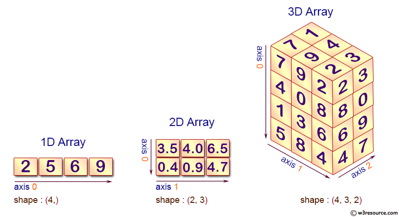
MegEngine provides a data structure called “tensor” ( Tensor ), which is different from the definition in mathematics, and its concept is the same as that in NumPy [1]: py:class:~numpy.ndarray is more similar, i.e. multidimensional arrays. Many unstructured data in the real world, such as text, pictures, audio, video, etc., can be abstracted into the form of Tensor for expression. The concept of Tensor we mentioned is often a generalization (or generalization) of other more specific concepts：

math	computer science	geometric concept	Concrete example
Scalar	Number	point	Score, probability
Vector	Array	String	List
Matrix	2 dimensional array (2d-array)	noodle	Excel spreadsheet
3-dimensional tensor	3-dimensional array (3d-array)	body	RGB pictures
…	…	…	…
n-dimensional tensor	n-dimensional array (nd-array)	high dimensional space

Taking a 2x3 matrix (a 2-dimensional tensor) as an example, initialize the Tensor with a nested Python list in MegEngine:

>>> Tensor([[1, 2, 3], [4, 5, 6]])
Tensor([[1 2 3]
 [4 5 6]], dtype=int32, device=xpux:0)

Its basic properties are Tensor.ndim, Tensor.shape, Tensor.dtype, Tensor.device and so on.

• We can perform various scientific calculations based on the Tensor data structure;

• Tensor is also the main data structure used in neural network programming. The input, output and conversion of the network are all represented by Tensor.

Note

The difference from NumPy is that MegEngine also supports the use of GPU devices for more efficient computations. When both GPU and CPU devices are available, MegEngine will preferentially use the GPU as the default computing device without requiring manual settings by the user. In addition, MegEngine also supports features such as automatic differentiation (Autodiff), which we will introduce in the appropriate sections of the subsequent tutorials.

If you have absolutely no experience with NumPy

• You can refer to the introduction in Deep understanding of Tensor data structure, or check the NumPy official website documentation and tutorials first;

• Other good supplementary material is ” Python Numpy Tutorial (with Jupyter and Colab) ” by CS231n.

Tensor operations and computations

Like NumPy’s multidimensional arrays, Tensor can perform element-wise addition, subtraction, multiplication, and division operations using standard arithmetic：.

>>> a = Tensor([[2, 4, 2], [2, 4, 2]])
>>> b = Tensor([[2, 4, 2], [1, 2, 1]])
>>> a + b
Tensor([[4 8 4]
 [3 6 3]], dtype=int32, device=xpux:0)
>>> a - b
Tensor([[0 0 0]
 [1 2 1]], dtype=int32, device=xpux:0)
>>> a * b
Tensor([[ 4 16  4]
 [ 2  8  2]], dtype=int32, device=xpux:0)
>>> a / b
Tensor([[1. 1. 1.]
 [2. 2. 2.]], device=xpux:0)

Tensor class provides some common methods, such as Tensor.reshape method, which can be used to change the shape of Tensor (this operation will not change the total number of Tensor elements and the value of each element)：

>>> a = Tensor([[1, 2, 3], [4, 5, 6]])
>>> b = a.reshape((3, 2))
>>> print(a.shape, b.shape)
(2, 3) (3, 2)

But usually we would Use Functional operations and calculations, for example use functional.reshape to change shape：

>>> import megengine.functional as F
>>> b = F.reshape(a, (3, 2))
>>> print(a.shape, b.shape)
(2, 3) (3, 2)

Warning

A common misconception is that beginners think that the shape of a itself will change after calling a.reshape(). In fact, this is not the case. Most operations in MegEngine are not in-place operations, which means that usually calling these interfaces will return a new Tensor without changing the original Tensor.

See also

functional module provides more operators, and divides the namespace according to the usage scenarios. At present, we only need to touch these most basic operators, and in the future, we will touch the specialized ones. Operators for neural network programming.

Understanding Computational Graphs

Note

• MegEngine is a deep neural network learning framework based on Computing Graph;

• In the field of deep learning, any complex deep neural network model can essentially be represented by a computational graph.

Let’s first introduce the basic concept of computational graph：by taking a simple mathematical expression \(y=w*x+b\) as an example

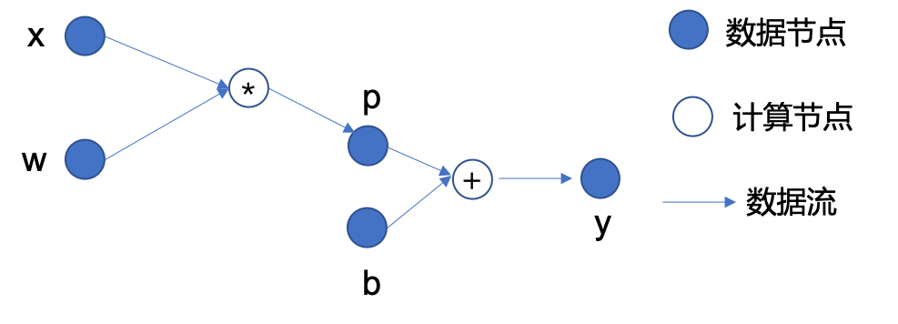
In MegEngine, Tensor is the data node, and Operator is the computing node

The node dependencies from input data to output data can form a directed acyclic graph (DAG), which has：

• Data node：as input data \(x\), parameters \(w\) and \(b\), intermediate result \(p\), and final output \(y\);

• In the calculation node：, \(*\) and \(+\) in the figure represent two operators of multiplication and addition, respectively, and calculate the output according to the given input;

• Directed edge：represents the flow of data, and reflects the front and back dependencies between data nodes and computing nodes.

With the representation of the computational graph, we can have a more intuitive understanding of the process of forward propagation and back propagation.

前向传播（Forward propagation）

The forward calculation is performed according to the definition of the model to obtain the output, which in the above example is -

1. Input data \(x\) and parameter \(w\) are multiplied to get intermediate result \(p\);

2. The intermediate result \(p\) and the parameter \(b\) are added to obtain the output result \(y\);

3. For more complex computational graph structures, the forward computation dependency is essentially a topological sort.

反向传播（Back propagation）

According to the target to be optimized (here we simply assume \(y\)), the gradient corresponding to all parameters in the model is obtained through the chain derivation rule. In the above example, \(\nabla y(w, b)\), consisting of partial derivatives \(\frac{\partial y}{\partial w}\) and \(\frac{\partial y}{\partial b}\).

This section will use calculus knowledge, which can be quickly learned/reviewed with the help of some materials on the：

3Blue1Brown - Essence of calculus [Bilibili] / Essence of calculus [YouTube]

For example, in order to get the partial derivative of \(y\) with respect to parameter \(w\) in the above figure, the process of backpropagation is shown in the following figure：

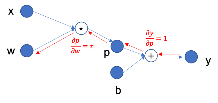
1. First there is \(y=p+b\), so \(\frac{\partial y}{\partial p}=1\);

2. Continue backpropagation, there are \(p=w*x\), so there is \(\frac{\partial p}{\partial w}=x\);

3. According to the chain rule \(\frac{\partial y}{\partial w}=\frac{\partial y}{\partial p} \cdot \frac{\partial p}{\partial w}=1 \cdot x\), so the final partial derivative of \(y\) with respect to parameter \(w\) is \(x\).

The obtained gradient will also be a Tensor, which will be used in the next step of parameter optimization.

参数优化（Parameter Optimization）

A common practice is to use gradient descent to update the parameters, in the above example to the values of \(w\) and \(b\). We use an example to help you understand the core idea of gradient descent：Suppose you are now lost in a valley and need to find a populated village, our goal is the lowest plain point (where the probability of being populated is the greatest). Adopting a gradient descent strategy requires us to look around each time to see which direction is the steepest; then take a step down in the negative direction of the gradient and cycle through the above steps, which we think can go downhill faster .

Every time we complete a parameter update, it means that the parameters have been iterated once, and there are often multiple iterations when training the model.

If you don’t know what gradient descent can achieve, that’s okay, there are more intuitive tasks practiced at the end of this tutorial. You can also find more material explaining the gradient descent algorithm on the Internet.

w, x, b = Tensor(3.), Tensor(2.), Tensor(-1.)

p = w * x
y = p + b

dydp = Tensor(1.)
dpdw = x
dydw= dydp * dpdw

>>> dydw
Tensor(2.0, device=xpux:0)

Automatic differentiation and parameter optimization

It is not difficult to find that with the chain rule, it is not difficult to calculate the gradient. But the computational graph we demonstrated above is only a very simple operation. When we use complex models, the abstracted computational graph structure will also become more complicated. If we manually calculate the gradient according to the chain rule at this time, The whole process will become extremely boring, and it is extremely unfriendly to careless friends, and no one wants to enter the long Debug stage because of a wrong calculation. Another feature of MegEngine as a deep learning framework is that it supports automatic differentiation, that is, it automatically completes the process of deriving parameter gradients according to the chain rule in the backpropagation process. At the same time, it also provides a corresponding interface to facilitate parameter optimization.

Tensor Gradients and Gradient Manager

In MegEngine, each Tensor has a property of Tensor.grad, which is short for Gradient.

>>> print(w.grad, b.grad)
None None

However, the above usage is incorrect. By default, Tensor does not calculate and record gradient information when calculating.

We need to use gradient manager GradManager to complete related operations：

• Use GradManager.attach to bind the parameters that need to calculate the gradient;

• Use the with keyword to record the entire forward calculation process to form a calculation graph;

• Call GradManager.backward for automatic backpropagation (automatic differentiation is done in the process).

from megengine.autodiff import GradManager

w, x, b = Tensor(3.), Tensor(2.), Tensor(-1.)
gm = GradManager().attach([w, b])
with gm:
    y = w * x + b
    gm.backward(y)

At this time, you can see the gradient corresponding to the parameters \(w\) and \(b\) ( \(\frac{\partial y}{\partial w} = x = 2.0\) was calculated earlier)：

>>> w.grad
Tensor(2.0, device=xpux:0)

Warning

It is worth noting that GradManager.backward calculates gradients by accumulating instead of replacing, if：is then executed

>>> # Note that `w.grad` is `2.0` now, not `None`
>>> with gm:
...     y = w * x + b
...     gm.backward(y)  # w.grad += backward_grad_for_w
>>> w.grad
Tensor(4.0, device=xpux:0)

It can be found that the gradient of parameter \(w\) is 4 instead of 2 at this time, this is because the new gradient and the old gradient are accumulated.

See also

For more details, see Basic principles and use of Autodiff .

Parameter

You may have noticed such a detail. In the previous introduction, we used parameters to call \(w\) and：b. Because unlike the input data :math:` :math:, they are required in the model training process. The variable to be updated by optimization. There are Parameter classes in MegEngine specifically to differentiate from Tensor, but it is essentially a special kind of tensor. Therefore, the gradient manager also supports maintaining the gradient information of Parameter in the calculation process.

from megengine import Parameter

x = Tensor(2.)
w, b = Parameter(3.), Parameter(-1.)

gm = GradManager().attach([w, b])
with gm:
    y = w * x + b
    gm.backward(y)

>>> w
Parameter(3.0, device=xpux:0)

>>> w.grad
Tensor(2.0, device=xpux:0)

Note

The difference between Parameter and Tensor is mainly reflected in the parameter optimization step, which will be introduced in the next section.

In the front we know the parameter \(w\) and its corresponding gradient \(w.grad\), the logic of performing a gradient descent is very simple：

\[w = w - lr * w.grad\]

Do the same for each parameter. A hyperparameter：learning rate is introduced here to control the magnitude of each parameter update. Different parameters can be updated with different learning rates, and even the same parameter can change the learning rate on the next update, but for ease of initial learning and understanding, we will use a consistent learning rate throughout the tutorial.

Optimizer

optimizer module of MegEngine provides optimizers based on various common optimization strategies, such as SGD and Adam, etc. Their base class is Optimizer, where SGD corresponds to the stochastic gradient descent algorithm, which is the optimizer that will be used in this tutorial.

import megengine.optimizer as optim

x = Tensor(2.)
w, b = Parameter(3.), Parameter(-1.)

gm = GradManager().attach([w, b])
optimizer = optim.SGD([w, b], lr=0.01)

with gm:
    y = w * x + b
    gm.backward(y)
    optimizer.step().clear_grad()

Call Optimizer.step for a parameter update, and call Optimizer.clear_grad to clear Tensor.grad.

>>> w
Parameter(2.98, device=xpux:0)

Many beginners tend to forget to clear the gradients on a new round of parameter updates, resulting in incorrect results.

Warning

Optimizer accepts input type must be Parameter instead of Tensor, otherwise an error will be reported.

TypeError: optimizer can only optimize Parameters, but one of the params is ...

See also

For more details, see Use Optimizer to optimize parameters.

Selection of optimization goals

To improve the prediction performance of the model, we need to have a suitable optimization objective.

But please note that the expression used for the example above is only used to understand the calculation graph, and its output value \(y\) is often not the object that actually needs to be optimized, it is only the output of the model, and it is meaningless to simply optimize this value .

So how do we evaluate the predictive performance of a model? The core principle is： **The less mistakes you make, the better you perform. **

Generally speaking, the objective we need to optimize is called the loss (Loss), which is used to measure the difference between the output value of the model and the actual result. If the loss can be optimized to be as low as possible, it means that the model predicts better on the current data. At present, we can assume that a model that performs well on the current dataset can also produce good predictions on newly input data.

Such a description may be a bit abstract, let us understand it directly through practice.

Exercise：Fitting a Line

Suppose you got the dataset \(\mathcal{D}=\{ (x_i, y_i) \}\), where \(i \in \{1, \ldots, 100 \}\), hope to give input \(x\) in the future , can predict the appropriate \(y\) value.

get_point_examples() 源码

Below is the code implementation to randomly generate these data points：

import numpy as np

np.random.seed(20200325)

def get_point_examples(w=5.0, b=2.0, nums_eample=100, noise=5):

    x = np.zeros((nums_eample,))
    y = np.zeros((nums_eample,))

    for i in range(nums_eample):
        x[i] = np.random.uniform(-10, 10)
        y[i] = w * x[i] + b + np.random.uniform(-noise, noise)

    return x, y

It can be found that the data points are generated based on the line \(y = 5.0 * x + 2.0\) plus some random noise.

But in this tutorial, we should assume that we don’t have such a God’s perspective, and all we can get is the coordinates of these data points, and we don’t know the ideal \(w=5.0\) and \(b=2.0\), only The parameters can be iteratively updated through the existing data. Use loss or other means to judge the quality of the final model (such as the fit of the straight line), and will show you a more scientific approach in subsequent tutorials.

>>> x, y = get_point_examples()
>>> print(x.shape, y.shape)
(100,) (100,)

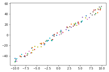
Through visual analysis, it is found (as shown above：that the distribution of these points is very suitable for fitting with a straight line \(f(x) = w * x + b\).

>>> def f(x):
...     return w * x + b

The abscissa \(x\) of all sample points will get a predicted output \(\hat{y} = f(x)\) after passing through our model.

In this tutorial, the gradient descent strategy we will adopt is Batch Gradient Descent, that is, at each iteration, the losses predicted on all data points are accumulated to obtain the overall loss and then averaged, which is used as the The optimization objective is to compute gradients and optimize parameters. The advantage of this is that the interference caused by noisy data points can be avoided, and each time the parameters are updated, they will be optimized in a more balanced direction. And from a computational efficiency point of view, you can take advantage of a feature called Vectorization to save time (verified in the extended material).

Design and implement a loss function

For such a model, how to measure the loss \(l\) between the output value \(\hat{y} = f(x)\) and the true value \(y\)? Please think along the following lines of thought：

1. The easiest way to think of it is to directly calculate the error (Error), that is, for every \((x_i, y_i)\) and \(\hat{y_i}\) there are \(l_i = l(\hat{y_i},y_i) = \hat{y_i} - y_i\).

2. This kind of thinking is natural, the problem is that for regression problems, the loss \(l_i\) obtained in the above form is positive and negative, when we calculate the average loss \(l = \frac{1}{n} \sum_{i}^{n} (\hat{y_i} - y_i)\) will cancel some positive and negative values, for example, for \(y_1 = 50, \hat{y_1} = 100\) and \(y2 = 50, \hat{y_2} = 0\), the average loss is \(l = \frac{1}{2} \big( (100 - 50) + (0 - 50) \big) = 0\), which is not what we want.

   We hope that the error on a single sample should be cumulative, so it needs to be positive while facilitating subsequent calculations.

3. An improvement to try is to use Mean Absolute Error (MAE): \(l = \frac{1}{n} \sum_{i}^{n} |\hat{y_i} - y_i|\)

   But note that we use gradient descent to optimize the model, which requires the objective function (ie, the loss function) to be as continuously derivable as possible, and easy to derive and calculate. So our more common loss function in regression problems is Mean Squared Error (MSE):

   \[l = \frac{1}{n} \sum_{i}^{n} (\hat{y_i} - y_i)^2\]

   Note

   • In some machine learning courses, for the convenience of derivation, the coefficient 2 brought by the square may be offset, and multiplied by \(\frac{1}{2}\) in front, which is not done in this tutorial (because MegEngine supports automatic derivation, which can be compared with manual Compare the code of the derivation process);

   • In addition, we can explain why MSE is chosen as the loss function： from the perspective of probability and statistics. Assuming that the error satisfies the normal distribution of the mean \(\mu = 0\), then MSE is the maximum likelihood estimation of the parameters. For a detailed explanation, see Lecture of CS229.

   If you don’t understand the above details, don’t worry, it won’t affect our task of completing this tutorial.

We assume that the prediction result pred on 4 samples is now obtained by the model, and now calculate the MSE loss：between it and the real value real

>>> pred = np.array([3., 3., 3., 3.])
>>> real = np.array([2., 8., 6., 1.])
>>> np_loss = np.mean((pred - real) ** 2)
>>> np_loss
9.75

Common loss functions are also encapsulated in MegEngine, here we can use square_loss:

>>> mge_loss = F.nn.square_loss(Tensor(pred), Tensor(real))
>>> mge_loss
Tensor(9.75, device=xpux:0)

Note：Since the loss function is a concept proposed in deep learning, the related interface should be called through functional.nn.

See also

• If you do not understand the above operations, please refer to Element-wise operations (Element-wise) or browse the corresponding API documentation;

• More common loss functions can be found at Loss functions.

Complete code implementation

We also give the NumPy implementation and the MegEngine implementation as a comparison：

• In the NumPy implementation, \(\frac{\partial l}{\partial w}\) and \(\frac{\partial l}{\partial b}\) need to be manually deduced, while in MegEngine just call gm. backward(loss) can;

• Input data \(x\) is a vector (1D array) of shape \((100,)\), when operating with scalars \(w\) and \(b\), the latter is broadcast to the same shape, and then calculate. In this way, the vectorization feature is used, and the calculation efficiency is higher. For details, please refer to Broadcast to Tensor .

NumPy

import numpy as np

x, y = get_point_examples()

w = 0.0
b = 0.0

def f(x):
    return w * x + b

nums_epoch = 5
for epoch in range(nums_epoch):

   # optimzer.clear_grad()
   w_grad = 0
   b_grad = 0

   # forward and calculate loss
   pred = f(x)
   loss = ((pred - y) ** 2).mean()

   # backward(loss)
   w_grad += (2 * (pred - y) * x).mean()
   b_grad += (2 * (pred - y)).mean()

   # optimizer.step()
   lr = 0.01
   w = w - lr * w_grad
   b = b - lr * b_grad

   print(f"Epoch = {epoch}, \
           w = {w:.3f}, \
           b = {b:.3f}, \
           loss = {loss:.3f}")

MegEngine

import megengine.functional as F
from megengine import Tensor, Parameter
from megengine.autodiff import GradManager
import megengine.optimizer as optim

x, y = get_point_examples()

w = Parameter(0.0)
b = Parameter(0.0)

def f(x):
    return w * x + b

gm = GradManager().attach([w, b])
optimizer = optim.SGD([w, b], lr=0.01)

nums_epoch = 5
for epoch in range(nums_epoch):
    x = Tensor(x)
    y = Tensor(y)

    with gm:
        pred = f(x)
        loss = F.nn.square_loss(pred, y)
        gm.backward(loss)
        optimizer.step().clear_grad()

    print(f"Epoch = {epoch}, \
            w = {w.item():.3f}, \
            b = {b.item():.3f}, \
            loss = {loss.item():.3f}")

Both should get the same output.

Since we are using a batch gradient descent strategy, each iteration (Iteration) is based on the average loss and gradient computed over all the data. In order to perform multiple iterations, we have to repeat the training multiple times (Epochs) (passing the data completely, called completing an Epoch training). Under the batch gradient descent strategy, only one Iter is updated for each training parameter. Later, we will encounter a situation where an Epoch iterates multiple times. These terms are very common in the communication in the field of deep learning and will be used in subsequent tutorials. mentioned repeatedly.

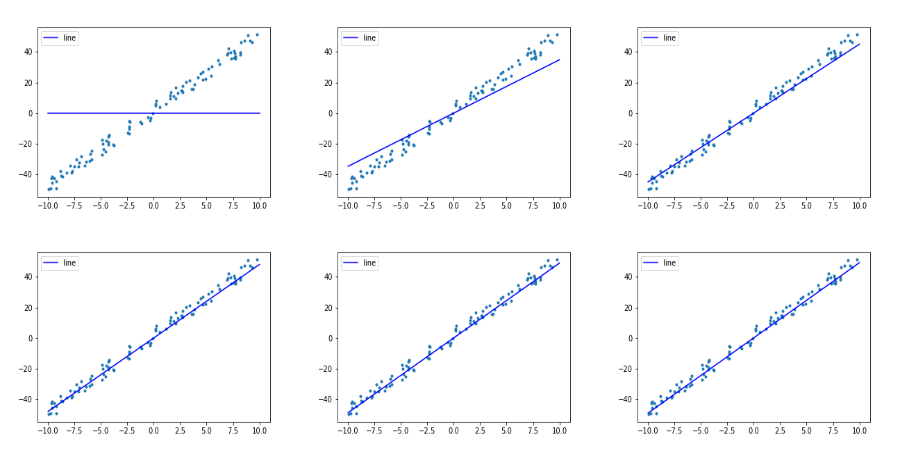
It can be found that after 5 epochs of training (5 iterations for a given task T), our loss is constantly decreasing, and the parameters \(w\) and \(b\) are also constantly changing.

Epoch = 0,             w = 3.486,             b = -0.005,             loss = 871.968
Epoch = 1,             w = 4.508,             b = 0.019,             loss = 86.077
Epoch = 2,             w = 4.808,             b = 0.053,             loss = 18.446
Epoch = 3,             w = 4.897,             b = 0.088,             loss = 12.515
Epoch = 4,             w = 4.923,             b = 0.123,             loss = 11.888

Through some visualization means, we can intuitively see that our straight line fitting degree is still very good.

This is a small step in our MegEngine journey, we have successfully completed the task of line fitting with MegEngine!

See also

The corresponding source code of this tutorial： examples/beginner/megengine-basic-fit-line.py

Summary：Unary Linear Regression

We try to use professional terms to define：regression analysis involving only two variables, called univariate regression analysis. If there is only one independent variable \(X\), and the quantitative relationship between the dependent variable \(Y\) and the independent variable \(X\) is approximately linear, a univariate linear regression equation can be established, from the independent variable \(X\) to predict the value of the dependent variable \(Y\), which is the univariate linear regression prediction. The univariate linear regression model \(y_{i}=\alpha+\beta x_{i}+\varepsilon_{i}\) is the simplest machine learning model and is great for getting started. The random disturbance term \(\varepsilon_{i}\) is a random variable that cannot be directly observed, that is, the noise introduced when we generate the data above. We learn \(w\) and \(b\) according to the existing data points, and get the sample regression equation \(\hat{y}_{i}= wx_{i}+b\) as a univariate linear regression prediction model.

The parameter estimation of the univariate linear regression equation usually uses the least squares method (also called the least squares method, Least squares method) to solve the form of the normal equation to obtain the closed-form expression. This method will not be introduced in this tutorial. ; The method we choose here is to use the gradient descent method to iteratively optimize the parameters. One is to show the use of basic functions in MegEngine such as GradManager and Optimizer, and the second is to be more natural in the future. In order to optimize the parameters of nonlinear models such as neural networks, the least squares method will no longer be applicable.

At this time, you can refer to Tom Mitchell’s definition of “machine learning” in “Machine Learning [2]”：

A computer program is said to learn from experience E with respect to some class of tasks T and performance measure P, if its performance at tasks in T, as measured by P, improves with experience E.

A computer program is said to have learned from experience E if it can improve its performance P on some class of tasks T based on experience E.

In this tutorial, our task T is to try to fit a straight line. The experience E comes from the data points we have. According to the distribution of data points, we naturally think of choosing a univariate linear model to predict the output. We evaluate the model well When it is bad (performance P), the MSE loss is used as the objective function, and the gradient descent algorithm is used to optimize the loss. In the next tutorial, we will be exposed to multiple linear regression models and gain a deeper understanding of machine learning concepts. Before that, you may need to spend some time digesting and absorbing the knowledge that has emerged, and practice a lot.

Tasks, Models and Optimization Algorithms

There are many types of models in the field of machine learning, and gradient descent is not the only optimization algorithm. We will be exposed to multiple linear regression models and linear classification models in later tutorials, transitioning from linear models to fully connected neural network models in deep learning; different models are suitable for different machine learning tasks, so model selection is very important . The models used in deep learning are called neural networks, and one of the： of neural networks is that they can be applied to many tasks, and sometimes achieve much better results than traditional machine learning models. However, its model structure is not complicated, and the process of optimizing the model is similar to this tutorial. Recall that any neural network model can be expressed as a computational graph, and we’ve already seen it for the first time.

Try tuning hyperparameters

We mentioned some concepts such as hyperparameters. Hyperparameters are parameters that need to be set manually and usually cannot be learned by the model itself. As you may have noticed, we are using the same learning rate for each iteration with parameters \(w\) and \(b\). After 5 iterations, the parameter \(w\) is very close to the ideal situation, and the parameter \(b\) needs to continue to be updated. Try changing the value of lr, or increase the number of Epoch for training, and see if the loss can be reduced further.

Does lower loss necessarily mean better?

Since we have chosen the loss as the optimization objective, ideally our model should fit as many points in the existing data as possible to reduce the loss. But the limitation is that the points we get are always training data, and for a machine learning task, we might use dataset A when training the model, and dataset B from the real world when actually using the model. At this time, optimizing the loss when training the model to the extreme may lead to overfitting.

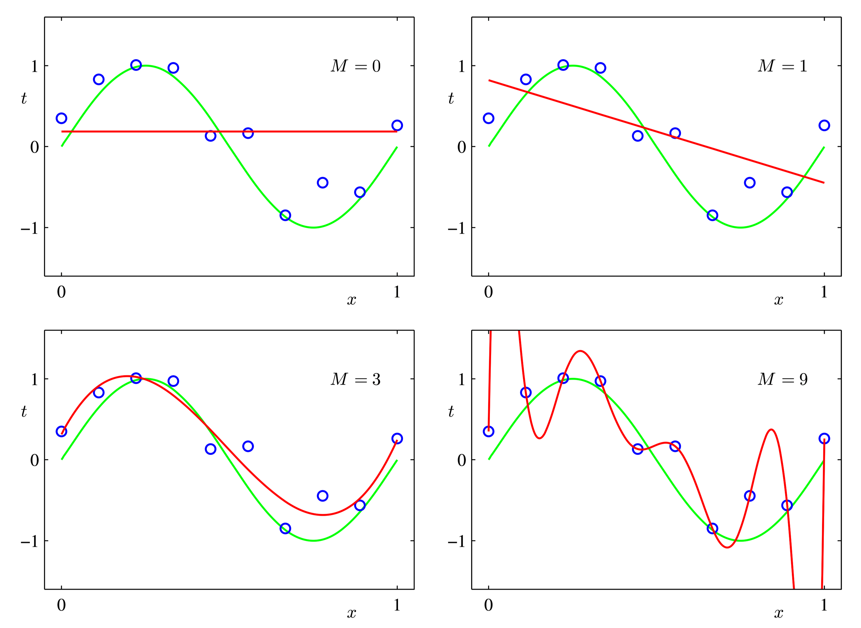
Christopher M Bishop Pattern Recognition and Machine Learning [3] - Figure 1.4

The distribution of data points in the above figure actually comes from the trigonometric function plus some noise. We choose a polynomial regression model and optimize it, hoping that the polynomial curve can fit the data points as much as possible. It can be found that when there are too many iterations, the last picture will appear. At this time, although the fitting degree on the existing data points has reached 100% (loss is 0), the prediction performance for the newly input data may not be as good as the early training situation. Therefore, the loss function in the training process cannot be used as an evaluation indicator for model performance.

We will give more scientific solutions in subsequent tutorials.

Expansion material

关于向量化优于 for 循环的简单验证

Inside：, vectorized operations are faster than for loops, and we can easily verify this.

import time

n = 1000000
a = np.random.rand(n)
b = np.random.rand(n)
c1 = np.zeros(n)

time_start = time.time()
for i in range(n):
    c1[i] = a[i] * b[i]
time_end = time.time()
print('For loop version:', str(1000 * (time_end - time_start)), 'ms')

time_start = time.time()
c2 = a * b
time_end = time.time()
print('Vectorized version:', str(1000 * (time_end - time_start)), 'ms')

print(c1 == c2)

For loop version: 460.2222442626953 ms
Vectorized version: 3.6432743072509766 ms
[ True  True  True ...  True  True  True]

Behind it is the use of SIMD for data parallelism. There are many blogs on the Internet that explain it in detail. It is recommended to read：

• Why is vectorization, faster in general, than loops?

• Nuts and Bolts of NumPy Optimization Part 1: Understanding Vectorization and Broadcasting

Likewise, vectorized code can be written faster in MegEngine than for loops, especially when using GPU parallelism.

Scikit-learn 文档：欠拟合和过拟合

Scikit-learn is a very well-known Python machine learning library that implements many classic machine learning algorithms. In Scikit-learn’s model selection documentation, code to explain model underfitting and overfitting is given：

https://scikit-learn.org/stable/auto_examples/model_selection/plot_underfitting_overfitting.html

Interested readers can take this to learn about Scikit-learn, we will use the dataset interface provided by it in the next tutorial.

references

[1]

Charles R. Harris, K. Jarrod Millman, Stéfan J. van der Walt, Ralf Gommers, Pauli Virtanen, David Cournapeau, Eric Wieser, Julian Taylor, Sebastian Berg, Nathaniel J. Smith, Robert Kern, Matti Picus, Stephan Hoyer, Marten H. van Kerkwijk, Matthew Brett, Allan Haldane, Jaime Fernández del Río, Mark Wiebe, Pearu Peterson, Pierre Gérard-Marchant, Kevin Sheppard, Tyler Reddy, Warren Weckesser, Hameer Abbasi, Christoph Gohlke, and Travis E. Oliphant. Array programming with NumPy. Nature, 585(7825):357–362, September 2020. URL: https://doi.org/10.1038/s41586-020-2649-2, doi:10.1038/s41586-020-2649-2.

[2]

Thomas M. Mitchell. Machine Learning. McGraw-Hill, Inc., USA, 1 edition, 1997. ISBN 0070428077.

[3]

Christopher M. Bishop. Pattern Recognition and Machine Learning (Information Science and Statistics). Springer-Verlag, Berlin, Heidelberg, 2006. ISBN 0387310738.