MegEngine implements neural network#
What this tutorial covers
Think about the limitations of linear models, consider how to solve the linear inseparability problem, and introduce the concept of “activation function”;
Have a basic understanding of neural and fully connected network model structures;
Expose to different parameter initialization strategies, learn to use
modulemodule to improve model design efficiency;According to the previous introduction, use MegEngine to implement a two-layer fully connected neural network to complete the Fashion-MNIST image classification task.
Get the original dataset#
In the last tutorial, we used MegEngine’s data.dataset module to obtain MNIST dataset and achieved over 90% classification accuracy using a linear classifier. Next, we will use the exact same model structure and optimization strategy on the similar Fashion-MNIST dataset to see if the linear model can still achieve the same good results.
Usually after 5 rounds of training, using a linear classifier (Logistic regression model) can achieve 83% accuracy on Fashion-MNIST.
Fashion-MNIST 数据集 + 线性分类器
Fashion-MNIST [1] is an image dataset that replaces the MNIST handwritten digits set. It is provided by the research division of Zalando, a German fashion technology company. It covers a total of 70,000 different product front images from 10 categories. The size, format, and train/test split of Fashion-MNIST are exactly the same as the original MNIST. 60000/10000 division of training and testing data, 28x28 grayscale images. You can use it directly to test the performance of your machine learning and deep learning algorithms without needing to change any code.
The source code of this part can be found in examples/beginner/linear-classification-fashion.py, the difference is:
MegEngine provides
MNISTinterface indata.datasetmodule, while Fashion-MNIST needs to be downloaded manually;Use the following
load_mnistfunction to get a data set in ndarray format, which needs to be encapsulated byArrayDataset.
import megengine
import megengine.data as data
import megengine.data.transform as T
import megengine.functional as F
import megengine.optimizer as optim
import megengine.autodiff as autodiff

def load_mnist(path, kind='train'):
    import os
    import gzip
    import numpy as np

    """Load MNIST data from `path`"""
    labels_path = os.path.join(path,
                               '%s-labels-idx1-ubyte.gz'
                               % kind)
    images_path = os.path.join(path,
                               '%s-images-idx3-ubyte.gz'
                               % kind)

    with gzip.open(labels_path, 'rb') as lbpath:
        labels = np.frombuffer(lbpath.read(), dtype=np.uint8,
                               offset=8)

    with gzip.open(images_path, 'rb') as imgpath:
        images = np.frombuffer(imgpath.read(), dtype=np.uint8,
                               offset=16).reshape(len(labels), 784)

    return images, labels


# Get train and test dataset and prepare dataloader
# Make sure that you have downloaded data and placed it in `DATA_PATH`
# GitHub link: https://github.com/zalandoresearch/fashion-mnist


from os.path import expanduser
DATA_PATH = expanduser("~/data/datasets/Fashion-MNIST")

X_train, y_train = load_mnist(DATA_PATH, kind='train')
X_test, y_test = load_mnist(DATA_PATH, kind='t10k')

mean, std = X_train.mean(), X_train.std()

train_dataset = data.dataset.ArrayDataset(X_train, y_train)
test_dataset = data.dataset.ArrayDataset(X_test, y_test)

train_sampler = data.RandomSampler(train_dataset, batch_size=64)
test_sampler = data.SequentialSampler(test_dataset, batch_size=64)

transform = T.Normalize(mean, std)

train_dataloader = data.DataLoader(train_dataset, train_sampler, transform)
test_dataloader = data.DataLoader(test_dataset, test_sampler, transform)

num_features = train_dataset[0][0].size
num_classes = 10


# Parameter initialization
W = megengine.Parameter(F.zeros((num_features, num_classes)))
b = megengine.Parameter(F.zeros((num_classes,)))


# Define linear classification model
def linear_cls(X):
    return F.matmul(X, W) + b


# GradManager and Optimizer setting
gm = autodiff.GradManager().attach([W, b])
optimizer = optim.SGD([W, b], lr=0.01)


# Training and validation
nums_epoch = 5
for epoch in range(nums_epoch):
    training_loss = 0
    nums_train_correct, nums_train_example = 0, 0
    nums_val_correct, nums_val_example = 0, 0

    for step, (image, label) in enumerate(train_dataloader):
        image = F.flatten(megengine.Tensor(image), 1)
        label = megengine.Tensor(label).astype("int32")

        with gm:
            score = linear_cls(image)
            loss = F.nn.cross_entropy(score, label)
            gm.backward(loss)
            optimizer.step().clear_grad()

        training_loss += loss.item() * len(image)

        pred = F.argmax(score, axis=1)
        nums_train_correct += (pred == label).sum().item()
        nums_train_example += len(image)

    training_acc = nums_train_correct / nums_train_example
    training_loss /= nums_train_example

    for image, label in test_dataloader:
        image = F.flatten(megengine.Tensor(image), 1)
        label = megengine.Tensor(label).astype("int32")
        pred = F.argmax(linear_cls(image), axis=1)

        nums_val_correct += (pred == label).sum().item()
        nums_val_example += len(image)

    val_acc = nums_val_correct / nums_val_example

    print(f"Epoch = {epoch}, "
          f"train_loss = {training_loss:.3f}, "
          f"train_acc = {training_acc:.3f}, "
          f"val_acc = {val_acc:.3f}")
You can use the following code to directly compare the difference between the two source code files:
cd examples/beginner
diff linear-classification.py linear-classification-fashion.py
Such results are not ideal compared to human level, and we need to design better machine learning models.
Limitations of Linear Models#
Linear models are simpler and therefore have many limitations. For example, when dealing with classification problems, the generated decision boundary is a hyperplane, which means that ideally, the sample points are linearly separable in the feature space. The most typical counter-example is that it cannot solve the exclusive-or (XOR) operation problem:
2D space representation
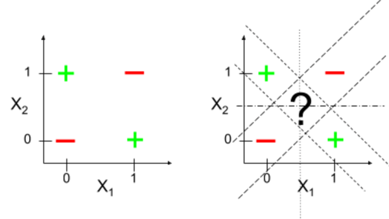
Since the data are linearly inseparable, we cannot find such a linear decision boundary that separates the two classes of samples well.
Note
We are about to transition from a linear model to a neural network model, and you will find that everything has already happened quietly.
Introduce nonlinear factors#
Recall that from the last tutorial, our linear classifier had an operation (link function) that maps linear predictions to probability values in the forward computation. Since this step of calculation has no effect on the decision boundary of the samples in the model, we can still consider this as a generalized linear model (a more terminological interpretation is that we assume that the observed samples still obey an exponential family distribution, which is not discussed in this tutorial. would go into too many mathematical details).
It’s time to tell you a secret. The linear model itself can be:of as the simplest single-layer neural network!

If the MNIST image sample flattened feature vector \(\boldsymbol{x}\) is regarded as the input layer (Input Layer), then for the binary classification problem, we can regard it as a neuron here, responsible for completing the linear prediction \(z= \boldsymbol{w}^T \boldsymbol{x} + b\) Calculations associated with link function \(a=\sigma(z)\). In binary classification problems, the output layer only needs one neuron to do the job, while multi-classification problems require multiple neurons.#
神经元计算模型,与生物学的联系
The basic computing unit of the brain is the neuron. About 86 billion neurons can be found in the human nervous system, which are connected with about \(10^{14}\) ~ \(10^{15}\) synapses. The figure below shows an example of a biological neuron (left) and a common mathematical model (right). Each neuron receives input signals from its dendrites (Dendrites) and produces output signals along its unique axon (Axon). The axons eventually branch out and connect to the synapses of other neurons through synapses. In a neuron computational model, a signal propagating along an axon (e.g. :math:` :math::math:w_0 x_0`). The synaptic strength (aka weight \(w\) ) is learnable and can control the degree of influence (and direction) of one neuron on another neuron, such as positive weights for excitation and negative weights for inhibition. In the basic model, dendrites transmit signals to the cell body, where the signals add up. If the final sum is above a certain threshold, the neuron will activate, outputting a spike to its axon.
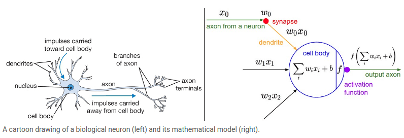
(Note:The explanations and pictures in this paragraph are quoted from <https://cs231n.github.io/neural-networks-1/>`section material 1`_ in the CS231n handout.)*
多分类问题,即意味着最终由多个神经元计算多个输出
For multi-classification problems, the single-layer neural network structure is shown below (it is assumed that the input data feature dimension is 16):

Each neuron in the output layer in the figure needs to complete linear computation and nonlinear mapping.
(Note:This image is generated using *`NN SVG <multilayer perceptron>`_.)*
Activation function and hidden layer#
In the neuron computing model, the nonlinear function is called the activation function (Activation function), and the activation function that is often used in history is the Sigmoid function we have seen \(\sigma(\cdot)\). This brings us to For inspiration, the activation function is nonlinear, which also means that nonlinearity is introduced into our computational model through the connections between the synapses of multiple neurons. We can do this by introducing a Hidden Layer:

There are 12 neurons in the hidden layer, and each neuron needs to be responsible for the corresponding nonlinear calculation and decide whether to activate or not.#
Let’s standardize the terminology, in the neural network model, the neural network above is called a 2-layer fully connected neural network. The input layer is a sample feature, and no actual calculation occurs, so it is not included in the number of model layers. There can be multiple hidden layers, and the number of neurons in each layer needs to be manually set. Since the neurons of the linear layer are completely connected with all the inputs of the previous layer, it is also called a fully connected layer (FC Layer). It is precisely because the activation function is added behind the fully connected layer that the neural network has the ability of nonlinear computing.
Use MegEngine to simulate this calculation process and feel it intuitively (only focus on shape changes here):
x = F.ones((16,))

W1 = F.zeros((16, 12))
b1 = F.zeros((12,))
z1 = F.matmul(x, W1) + b1  # Linear (full connected)
a1 = F.nn.sigmoid(z1)  # Activations

W2 = F.zeros((12, 10))
b2 = F.zeros((10))
z2 = F.matmul(a1, W2) + b2  # Linear (full connected)
output = F.softmax(z2)  # Logits
>>> output.shape
(10,)
In MegEngine, common nonlinear activation functions are implemented in the functional.nn module. Since there may be a large number of nonlinear calculations in the neural network, and unlike the classifier, which requires the output to be mapped to the probability interval, the more commonly used activation functions are the sigmoid function, it has the characteristics of simple calculation and derivation, and meets the characteristic requirements of nonlinear calculation. For a more specific explanation, check out the API documentation for the different activation functions.
In the field of deep learning, there are many researches and designs on activation functions. For the convenience of this tutorial, the ReLU activation function is used.
Multilayer Neural Network#
In addition to the selection of the activation function, the steps to define a fully connected neural network are mainly to design the number of hidden layers and the number of neurons in each layer.
We can make the model have stronger learning ability and expressive ability by stacking more hidden layers. From this point of view, the transformation in the linear model (accurately speaking, the affine transformation, but here we emphasize the difference between nonlinear and linear), no matter how superimposed, can finally be represented by an equivalent transformation, that is, a matrix The form of \(C=AB\) in arithmetic. Although we introduce nonlinearity through the activation function, the problem also arises:
We need to manage more model parameters, the solution in MegEngine will be given in this tutorial;
Neural network models can theoretically approximate arbitrary functions, and using deeper networks usually means stronger approximation capabilities. But we can’t design randomly, and we also need to make trade-offs between the amount of parameters in the model (the amount of calculation) and the final performance of the model.
See also
At present, the neural network model architecture that is only composed of fully connected layers (and activation functions) is also called Multilayer perceptron (MLP) in some materials. The starting point is to improve the perceptron algorithm, and then get the MLP. The two essentially refer to the same. We use Logistic regression to solve the binary classification problem, so we do not use the term perceptron.
random initialization strategy#
We need to pay attention to some characteristics of fully connected layers, such as each neuron in the layer will operate with all the inputs in the previous layer. Recall that when we introduced the linear model, we mentioned that the parameters in the model will be iteratively optimized from an initial value, and the simplest initialization strategy is adopted, all-zero initialization, that is, the values of all parameters in the model are initialized to 0 . This approach works in the case of single-layer model output + loss function, but will cause problems for multi-layer neural networks.
Suppose we initialize all the neuron parameters in the hidden layer to zero, which actually means that all the neurons are doing the same:
During forward calculation, since the input of the previous layer is the same, the output of the forward calculation of the neurons in the same layer will be the same;
When passing through the activation function, since the activation function ReLU has no randomness, the same output will be obtained and passed to the next layer;
In reverse calculation, all parameters will get the same gradient, and if the learning rate is the same, the parameters will be the same after updating.
This results in that all neurons in the fully connected layer are doing the same thing, and the ability to express is greatly reduced. The solution is to use a random initialization strategy.
MegEngine generates random data
random module is provided in MegEngine to randomly generate Tensor:
import megengine.random as rand

rand.seed(20200325)
x = rand.normal(0, 1, (3, 3))
>>> x
Tensor([[ 0.014   0.3366  0.877 ]
[ 0.4073 -0.0031  0.2638]
[-0.1826  1.4192  0.2758]], device=xpux:0)
Among them, random.seed can set a random seed, which is convenient to reproduce the random state in some cases. We randomly generated a Tensor of shape \((3, 3)\) from a standard normal distribution (mean 0, standard deviation 1) using the normal interface.
当模型变复杂后,重复的编码模式出现了
Suppose we need to add a hidden layer:with 256 neurons to the original linear classification model
num_features = train_dataset[0][0].size
num_hidden = 256
num_classes = 10

W1 = megengine.Parameter(rand.normal(0, 1, (num_features, num_hidden)))
b1 = megengine.Parameter(F.zeros((num_hidden,)))
W2 = megengine.Parameter(rand.normal(0, 1, (num_hidden, num_classes)))
b2 = megengine.Parameter(F.zeros((num_classes,)))

def model(X):
    z1 = F.matmul(X, W1) + b1
    a1 = F.nn.relu(z1)
    z2 = F.matmul(a1, W2) + b2
    return z2

gm = autodiff.GradManager().attach([W1, W2, b1, b2])
optimizer = optim.SGD([W1, W2, b1, b2], lr=0.1)
It can be clearly felt that when the model structure becomes more and more complex, the code will be filled with a lot of repetitive content.
As a deep learning framework, MegEngine naturally needs to provide a convenient way to design models.
Use Module to define the model#
See also
The introduction of this section of this tutorial is relatively concise, please refer to Use Module to define the model structure for the complete content.
The module module in MegEngine provides a class of abstract mechanism for the structure in the neural network model, everything is Module class, except for the implementation of the default random initialization strategy for common modules, And provides common methods (such as the upcoming Module.parameters). This allows users to focus on designing the network structure, freeing them from details such as repetitive parameter initialization and management methods.
For example, for a linear layer operation like matmul, you can use Linear to represent:
import megengine.module as M

x = F.ones((num_features,))  # (784,)
fc = M.Linear(num_features, num_hidden)  # (784, 256)
It can be found that the fc module has the weight (Weight) and bias (Bias) parameters of the corresponding shape, and the initialization is automatically completed.
>>> fc.weight.shape
(256, 784)
>>> fc.bias.shape
(256,)
According to the API documentation, for the input sample \(x\), the calculation process is \(y=xW^T+b\).
Simply verify that the operation result of Linear is consistent with the result obtained by matmul (within the floating point error range):
>>> a = fc(x)
>>> b = F.matmul(x, fc.weight.transpose()) + fc.bias
>>> print(a.shape, b.shape)
(256,) (256,)
>>> a - b < 1e-6
Tensor([ True  True  True  True  True  True  True  True  True  True  True  True
  True  True  True  True  True  True  True  True  True  True  True  True
  True  True  True  True  True  True  True  True  True  True  True  True
  True  True  True  True  True  True  True  True  True  True  True  True
  True  True  True  True  True  True  True  True  True  True  True  True
  True  True  True  True  True  True  True  True  True  True  True  True
  True  True  True  True  True  True  True  True  True  True  True  True
  True  True  True  True  True  True  True  True  True  True  True  True
  True  True  True  True  True  True  True  True  True  True  True  True
  True  True  True  True  True  True  True  True  True  True  True  True
  True  True  True  True  True  True  True  True  True  True  True  True
  True  True  True  True  True  True  True  True  True  True  True  True
  True  True  True  True  True  True  True  True  True  True  True  True
  True  True  True  True  True  True  True  True  True  True  True  True
  True  True  True  True  True  True  True  True  True  True  True  True
  True  True  True  True  True  True  True  True  True  True  True  True
  True  True  True  True  True  True  True  True  True  True  True  True
  True  True  True  True  True  True  True  True  True  True  True  True
  True  True  True  True  True  True  True  True  True  True  True  True
  True  True  True  True  True  True  True  True  True  True  True  True
  True  True  True  True  True  True  True  True  True  True  True  True
  True  True  True  True], dtype=bool, device=xpux:0)
Module 参数初始化策略
Linear As a built-in Module, we don’t need to initialize it manually, this process has been implemented in its corresponding __init__ method, and it is also allowed to be implemented by users themselves overwrite. Some common initialization strategies are provided in the module.init module and will not be covered in detail in this tutorial.
Module allows nested implementations like building blocks, so the fully connected neural network in this tutorial can be implemented:this.
All network structures are derived from the base class
M.Module. In the constructor, you must first callsuper().__init__().In the constructor, declare all layers/modules to be used;
In the
forwardfunction, define how the model will run, from input to output.
class NN(M.Module):
   def __init__(self):
      super().__init__()
      self.fc = M.Linear(num_features, num_hidden)
      self.classifier = M.Linear(num_hidden, num_classes)

   def forward(self, x):
      x = F.nn.relu(self.fc(x))
      x = self.classifier(x)
      return x
An iterator of model parameters can be obtained with the help of Module.parameters, which is provided to the gradient manager and optimizer:
>>> gm = autodiff.GradManager().attach(model.parameters())
>>> optimizer = optim.SGD(model.parameters(), lr=0.01)
Practice:Feedforward Neural Networks#
A feedforward neural network is the simplest type of neural network. Each neuron is arranged in layers, and each neuron is only connected to the neurons in the previous layer. Receive the output of the previous layer and output it to the next layer without feedback between layers. It is one of the most widely used and fastest-growing artificial neural networks.
In short, the feedforward neural network contains no other types of structures except the fully connected layer Linear, let’s implement it with MegEngine:
import megengine
import megengine.data as data
import megengine.data.transform as T
import megengine.functional as F
import megengine.module as M
import megengine.optimizer as optim
import megengine.autodiff as autodiff

def load_mnist(path, kind='train'):
    import os
    import gzip
    import numpy as np

    """Load MNIST data from `path`"""
    labels_path = os.path.join(path,
                               '%s-labels-idx1-ubyte.gz'
                               % kind)
    images_path = os.path.join(path,
                               '%s-images-idx3-ubyte.gz'
                               % kind)

    with gzip.open(labels_path, 'rb') as lbpath:
        labels = np.frombuffer(lbpath.read(), dtype=np.uint8,
                               offset=8)

    with gzip.open(images_path, 'rb') as imgpath:
        images = np.frombuffer(imgpath.read(), dtype=np.uint8,
                               offset=16).reshape(len(labels), 784)

    return images, labels


# Get train and test dataset and prepare dataloader
# Make sure that you have downloaded data and placed it in `DATA_PATH`
# GitHub link: https://github.com/zalandoresearch/fashion-mnist

from os.path import expanduser
DATA_PATH = expanduser("~/data/datasets/Fashion-MNIST")

X_train, y_train = load_mnist(DATA_PATH, kind='train')
X_test, y_test = load_mnist(DATA_PATH, kind='t10k')

mean, std = X_train.mean(), X_train.std()

train_dataset = data.dataset.ArrayDataset(X_train, y_train)
test_dataset = data.dataset.ArrayDataset(X_test, y_test)

train_sampler = data.RandomSampler(train_dataset, batch_size=64)
test_sampler = data.SequentialSampler(test_dataset, batch_size=64)

transform = T.Normalize(mean, std)

train_dataloader = data.DataLoader(train_dataset, train_sampler, transform)
test_dataloader = data.DataLoader(test_dataset, test_sampler, transform)

num_features = train_dataset[0][0].size
num_hidden = 256
num_classes = 10


# Define model
class NN(M.Module):
    def __init__(self):
        super().__init__()
        self.fc = M.Linear(num_features, num_hidden)
        self.classifier = M.Linear(num_hidden, num_classes)

    def forward(self, x):
        x = F.nn.relu(self.fc(x))
        x = self.classifier(x)
        return x


model = NN()

# GradManager and Optimizer setting
gm = autodiff.GradManager().attach(model.parameters())
optimizer = optim.SGD(model.parameters(), lr=0.01)


# Training and validation
nums_epoch = 5
for epoch in range(nums_epoch):
    training_loss = 0
    nums_train_correct, nums_train_example = 0, 0
    nums_val_correct, nums_val_example = 0, 0

    for step, (image, label) in enumerate(train_dataloader):
        image = F.flatten(megengine.Tensor(image), 1)
        label = megengine.Tensor(label).astype("int32")

        with gm:
            score = model(image)
            loss = F.nn.cross_entropy(score, label)
            gm.backward(loss)
            optimizer.step().clear_grad()

        training_loss += loss.item() * len(image)

        pred = F.argmax(score, axis=1)
        nums_train_correct += (pred == label).sum().item()
        nums_train_example += len(image)

    training_acc = nums_train_correct / nums_train_example
    training_loss /= nums_train_example

    for image, label in test_dataloader:
        image = F.flatten(megengine.Tensor(image), 1)
        label = megengine.Tensor(label).astype("int32")
        pred = F.argmax(model(image), axis=1)

        nums_val_correct += (pred == label).sum().item()
        nums_val_example += len(image)

    val_acc = nums_val_correct / nums_val_example

    print(f"Epoch = {epoch}, "
          f"train_loss = {training_loss:.3f}, "
          f"train_acc = {training_acc:.3f}, "
          f"val_acc = {val_acc:.3f}")
See also
The corresponding source code of this tutorial: examples/beginner/neural-network.py
After 5 rounds of training, a neural network model with an accuracy rate of over 83% (linear classifier) is usually obtained. In this tutorial we just want to demonstrate that introducing nonlinearity into the model leads to better expressiveness and predictive performance, so we didn’t spend time tuning hyperparameters and continuing to optimize our model. The Fashion-MNIST dataset officially maintains a `benchmark test <http://fashion-mnist.s3-website.eu-central-1.amazonaws.com/>result. It can be found that there are test results obtained by using MLPClassifier, which can reach 87.7%. We can reproduce the model and experimental results according to the description of the relevant model. A neural network model with comparable performance is obtained.
In fact, from the moment we touch the neural network model, we have already started to enter the “tuning hyperparameters” mode. Neural network models require the right code and hyperparameter design to achieve very good results. For MegEngine beginners who have just come into contact with neural networks, trying more coding is the most recommended way to improve. Inside the Megvii Technology Research Institute, the process of training a model is called “alchemy”, and now this term has become an industry slang. In the process of completing the MegEngine introductory tutorial, you are actually accumulating the most basic alchemy experience.
Summary:and then explore the calculation diagram#
We mentioned computational graphs in the first tutorial, now let’s recall:
MegEngine is a deep neural network learning framework based on Computing Graph;
In the field of deep learning, any complex deep neural network model can essentially be represented by a computational graph.
When we run the neural network model training code in this tutorial, we can further imagine in our minds, what should this fully connected neural network be expressed as a computational graph? When we visualize the structure of a neural network model, we usually focus on the change process of data nodes, but the computing nodes, or operators, in the calculation graph are also very critical. Assuming that our operator can only be a linear operation such as matmul / Linear, then the model will also impose restrictions on the shape of the input data, which must be expressed as a feature vector ( i.e. a 1-d tensor). When we face more complex data representation forms, such as RGB 3-channel color images, can we continue to use fully connected neural networks?
In the next tutorial we will experiment with the CIFAR 10 color image dataset and see if a fully connected network works. At that time, we will introduce a new operator (keep it mysterious for now), and find that designing a neural network is actually like building blocks, there will be many different effective structures, which are suitable for different scenarios, and when designing an operator , some traditional domain knowledge can sometimes be helpful.
Expansion material#
3Blue1Brown 关于深度学习的可视化介绍视频
We have used the form of visualization to understand the basic representation of grayscale images in computer vision. Visualization is an effective aid for us to understand data, or even understand a new knowledge and concept. I believe you already understand the basic concepts of deep learning including “Fully Connected Neural Network (Multilayer Perceptron)”, “Gradient Descent”, “Backpropagation”, and 3Blue1Brown’s video can be a very good supplement:
More Deep Learning Videos from 3Blue1Brown
`The structure of deep learning neural network <https://www.bilibili.com/video/BV1bx411M7Zx>
`Intuitive understanding of deep learning back propagation <https://www.bilibili.com/video/BV16x411V7Qg>
在 Kaggle 上使用全连接神经网络刷点吧!
Classic datasets such as MNIST and FashionMNIST are also available on Kaggle, you can try to use MegEngine to implement a fully connected neural network model, try to adjust the model structure (number of layers, number of neurons per layer) and Hyperparameters (learning rate, number of training rounds, etc.), try your best to increase the accuracy percentage on these two data sets, and feel the charm of alchemy.
There are also many other openly written code in Kaggle, which is a very good learning and reference material. You may see some people get better results using another model called “Convolutional Neural Networks”, and that’s what we’ll be covering in the next tutorial.
异或问题,人工智能的第一次寒冬
You may have heard the introduction to the history of artificial intelligence development in many materials, and it must mention several cold winters of artificial intelligence.
“The perceptron can’t solve the XOR problem!” This was a turning point in history.
Perceptron This is an artificial neural network developed in the late 1950s and early 1960s, psychologist Frank Rosenblatt released the first “perceptron” model in 1957, Marvin Minsky and Seymour Papert in 1969 Published “Introduction to Perceptron:Computational Geometry” to commemorate. But the perceptron is pessimistically predicted in this book, it can’t solve even the simplest classification (XOR) problem! This led to a shift in the direction of AI research at the time, leading to the AI winter of the 1980s.
Try it out and design the simplest possible XOR neural network model, which requires getting the output exactly right.
(Note:If you are interested, you can learn about the development history of artificial intelligence. Some documentaries and articles are quite fascinating.)
没有 Autodiff, Optimizer 和 Module 的话,将会是什么样子?
One of the most effective ways to learn something is to implement it yourself (even the Naive version), which is harder and more time consuming.
You can try to implement a fully connected neural network entirely in NumPy (there are many examples of this on the Kaggle platform), not too complicated, just two layers. You can choose to refer to the existing design in MegEngine to implement, or you can use it completely. It is not required to implement an automatic differentiation system, and the ``backward’ logic of each operator can be implemented manually; nor does it require the use of GPU for acceleration (after all, a lot of additional knowledge is required, such as Nvidia’s CUDA programming).