MegEngine implements linear regression#
What this tutorial covers
Understand the concepts related to data (Data) and data set (Dataset) in machine learning, and use MegEngine to encapsulate it;
Understand Mini-batch Gradient Descent, and the basic usage of
DataLoader;According to the previous introduction, use MegEngine to complete the housing price prediction task of the California housing dataset.
In this tutorial, you will be exposed to more interfaces of Tensor operations and operations
Some knowledge of linear algebra is required, the following materials are used to review when reading the:
Kaare Brandt Petersen - `The Matrix Cookbook <https://www.math.uwaterloo.ca/~hwolkowi/matrixcookbook.pdf>
3Blue1Brown - Essence of linear algebra [Bilibili] / Essence of linear algebra [YouTube]
Changed in version 1.7: The dataset used in this tutorial has been replaced by the Boston housing dataset with the California housing dataset.
Get the original dataset#
In the last tutorial ” MegEngine basic concepts “, we tried to fit a straight line with MegEngine. But in the real world, the tasks we face may not be so simple, and the representation of data is not so straightforward and abstract. Therefore, in this tutorial, we will complete a more complex linear regression task, which will use the `California Housing Dataset <https://www.dcc.fc.up.pt/~ltorgo/Regression/cal_housing.html>to complete the house price prediction task.
We will use the interface to Scikit-learn (please install it yourself) to get California housing data:
from sklearn.datasets import fetch_california_housing
from os.path import expanduser

DATA_PATH = expanduser("~/data/datasets/california")

X, y = fetch_california_housing(data_home=DATA_PATH, return_X_y=True)
Note:The dataset will be obtained from StatLib, please ensure that you can access the website normally. The resulting X and y will be in NumPy’s ndarray format.
There are many public datasets in the community for our study and research, so many Python libraries will encapsulate the interface to obtain some datasets, which is convenient for users to call. We’ll also see the .data.dataset module provided in :mod:in subsequent tutorials, which provides similar functionality.
>>> print(X.shape, y.shape)
(20640, 8) (20640,)
Learn about dataset information#
Recall that in the previous tutorial, our input data shape was \((100, )\), which means there are 100 samples in total, and each sample contains only one independent variable, so it is also called univariate linear regression; and here we get \(X\) has a shape of \((20640, 8)\), indicating that there are 20640 samples in total, what does the latter 8 mean? It is easy to think that there are 8 independent variables here, that is, we will use the multiple linear regression model to complete the housing price prediction.
California Housing 数据集
Consult the California Housing dataset document to know that there are: total of 20640 examples (Instances) in the California Housing dataset, and each example includes 8 attributes (Attributes). The attribute information is as follows:
MedInc: median income in block groupHouseAge: median house age in block groupAveRooms: average number of rooms per householdAveBedrms: average number of bedrooms per householdPopulation: block group populationAveOccup: average number of household membersLatitude: block group latitudeLongitude: block group longitude
Each attribute is represented by a specific value and informs us that there are no missing attribute values.
Processes intentionally missing from this tutorial
Users who have experience in machine learning or data mining projects may know that we usually perform Exploratory Data Analysis (EDA) on the raw data obtained to help us better perform feature engineering and select models later. Interested readers can understand by themselves, but these steps are not the focus of this tutorial, and introducing these processes will increase the difficulty of learning.
Data related concepts#
We have a preliminary understanding of the relevant information of the California housing data set, and then we can explore the related concepts of data (Data).
In order for computers to help us solve real-world problems, we need to model the problem and abstract it into a form that the computer can easily understand. We already know that machine learning is learning from data (Learning from data), so the representation of data is critical. When we describe a thing, we usually look for its attributes (Attribute) or features (Feature):
For example, when we describe the appearance of a Shiba Inu, we will say how the Shiba’s nose, ears, hair, etc.;
Another example is in video games, the attributes of characters often include health, magic, attack, defense and other attributes;
In the computer, all this information needs to be represented by discrete data, and the most common way is to quantify it into numerical values.
弃用波士顿房屋数据集的原因 - 机器学习的伦理问题
We used the Boston housing dataset for the house price prediction task in an old tutorial, but it is now deprecated. As surveyed in the paper racist data destruction? , the authors of this dataset designed an irreversible variable “B” assuming that apartheid had a positive effect on house prices. Such datasets are ethically controversial and should not be widely used.
Although the data set is replaced, the focus in this tutorial is not whether the selection of data features is scientific, but the situation where the:of features increases.
>>> X[0]  # a sample
array([   8.3252    ,   41.        ,    6.98412698,    1.02380952,
        1.          ,    2.55555556,   37.88      , -122.23      ])
Each example in the housing dataset is also called a sample, so the sample size \(n\) is 20640. The property information recorded in each sample can be represented by a feature vector \(\boldsymbol{x}=\left (x_{1}, x_{2}, \ldots, x_{d}\right)\) to indicate that each element in it corresponds to a certain dimension feature of the sample, we abbreviate the dimension of the feature as \(d\), its value is 8. Therefore, our dataset can be represented by a data matrix \(X\), and the prediction target is also called a label (Label):
where \(x_{i,j}\) represents the \(j\) dimension feature of the \(i\) sample, scalar \(y_i\) is the label value corresponding to sample \(\boldsymbol{x}_{i}\), \((\boldsymbol{x}, y)\) forms the Example. When performing matrix operations, the vector defaults to a column vector
A discussion of computing the multiplication form of:#
Our task is to predict house prices using a linear regression model \(Y=X \beta+\varepsilon\), where \(\varepsilon\) is a random perturbation. The difference from univariate linear regression is that there are multiple independent variables \(x\) at this time, our parameter \(\boldsymbol{w}\) is also changed from a scalar to a vector, for a single sample \(\boldsymbol{x}\) has:
The dot product of the two vectors will result in a scalar that, when added to the scalar \(b\), is the predicted house price.
In MegEngine, the interface for vector dot product operations is functional.dot:
import megengine
import megengine.functional as F

n, d = X.shape
x = megengine.Tensor(X[0])
w = F.zeros((d, ))
b = 0.0

y = F.dot(w, x) + b
>>> print(y, y.shape)
Tensor(0.0, device=xpux:0) ()
To take advantage of vectorization (to avoid writing out for loops), we want to have:for the entire batch of data \(X\)
:func:The numpy.dot interface in NumPy does support dot-by-:between n-dimensional arrays and 1-dimensional arrays (vectors)
import numpy as np

w = np.zeros((d,))
b = 0.0
y = np.dot(X, w) + b
>>> y.shape
(20640,)
MegEngine 中的 dot 不支持矩阵与向量相乘
Read the API documentation of ` :func:to find that it supports dot product operations with various input forms.
If the input \(a\) and \(b\) are both 1-dimensional arrays (vectors), equivalent to the inner product
numpy.inner;If the input \(a\) and \(b\) are both 2-dimensional arrays (matrices), equivalent to matrix multiplication
numpy.matmulor the infix operator@;If one of the inputs \(a\) and \(b\) is a 0-dimensional array (scalar), equivalent to element-wise multiplication
numpy.multiplyor the infix operator*;If input \(a\) is an n-dimensional array, and input \(b\) is a 1-dimensional array, the sum product will be calculated on the last axis of \(a\) and \(b\);
if…
It can be seen that this numpy.dot interface is a bit too versatile. If the user does not consult the documentation, it is difficult to think of the specific behavior when calling it, which is inconsistent with the interface design philosophy of MegEngine. MegEngine emphasizes transparent syntax and explicit behavior, and tries to avoid storage, ambiguity and misuse. Therefore, functional.dot refers to the dot product of vectors, and does not support input of other shapes.
This also means that interfaces with the same or similar names do not represent exactly the same definition and implementation logic. We can also refer to Dot product in MARLAB and find that the definition is not exactly the same as that of NumPy.
The interface for matrix multiplication in MegEngine is functional.matmul, corresponding to the infix operator @.
The official Python proposal PEP 465 provides discussion and recommended semantics for a dedicated infix operator @ for matrix multiplication, compatible with input forms of different shapes. It is mentioned that for a 1-dimensional vector input, it can be promoted to a 2-dimensional matrix by appending a dimension of length 1, and after performing the matrix multiplication operation, the temporarily added dimension is removed from the input. This makes both matrix@vector and vector@matrix legal operations (assuming compatible shapes), and both return a 1D vector.
Taking this multiple linear regression model as an example, its calculation method becomes :math:in MegEngine Y=XW+B:
>>> X = megengine.Tensor(X)
>>> W = F.expand_dims(F.zeros(d, ), 1)
>>> b = 0.0
>>> y = F.squeeze(F.matmul(X, W) + b)
>>> y.shape
(20640,)
Through the
expand_dimsinterface, we turn a zero vector \(w\) of shape \((d,)\) into a column vector \(W\) of shape \((d,1)\);Through the
matmulinterface, perform matrix multiplication \(P=XW\), \(P\) is the intermediate calculation result;When doing \(Y=P+b\), scalar \(b\) broadcasts a shape-compatible column vector \(B\);
Through the
squeezeinterface, the redundant dimension is removed, and \(Y\) is changed back to the vector \(y\).
Although the functions of expand_dims and squeeze can also be achieved by reshape, but for code readability, we should use as much as possible when there is a dedicated interface These are interfaces with transparent semantics.
MegEngine’s matmul is also compatible with non-matrix input:due to the existence of the recommended definition of PEP 465
>>> X = megengine.Tensor(X)
>>> w = F.zeros((d,))
>>> y = F.matmul(X, w) + b
>>> y.shape
(20640,)
为什么 matmul 兼容不同类型的形状
Compatibility with different input shapes makes local matrix multiplication code very easy to write in high-dimensional cases without compromising code readability.
Although this may conflict with the MegEngine interface design philosophy, compatibility with community-consistent standards is a minimum requirement. The representation of matrix multiplication has been widely discussed and practically verified in the Python data science community for a long time, and finally a consensus has been reached. This is the official reference provided at the Python language level, and the numpy.dot interface design in NumPy has not been unanimously recognized by the community.
Now that we have implemented a sufficiently vectorized code, it appears that the gradient descent algorithm can be used to optimize the model parameters.
Several forms of gradient descent#
If for each input sample, we calculate the loss and update the model parameters in time, the parameter iteration frequency will be very high - this method is called Stochastic Gradient Descent (SGD), also known as Online Gradient Descent (Online Gradient Descent) Gradient Descent), this form of gradient descent is very easy to understand. The problem is that frequent updates will cause the change of gradient to jump (the direction is unstable); in addition, multiple loop operations are required during the entire training process. If the scale of data becomes huge, this form of calculation will become very low. effect.
We have emphasized many times in the tutorial that:should be written in vectorized form instead of for loop form to pursue higher computational efficiency. Therefore, when we calculate forward, we usually choose to use batch data as input instead of a single sample, which is actually the idea of parallel computing. In addition to this reason, batch gradient descent can also reduce the interference caused by abnormal data, iterate parameters in the direction of overall better, and the loss converges more stably.
But batch gradient descent also has its own limitations. Overly stable gradient changes can cause the model to prematurely converge to a less-than-ideal set of parameters. Our strategy of accumulating gradients may also introduce other uncertainties that affect the entire training process. Considering the large-scale data input situation, it is very likely that we cannot load the entire data set into memory at one time; even if the memory capacity problem is solved, batch gradient descent is performed on large data sets, and the speed of parameter iterative update will be significantly slow down.
What is easily overlooked is the process of converting NumPy ndarrays to:Tensors. There is actually data handling here.
>>> X = megengine.Tensor(X)
Weighing the pros and cons between stochastic gradient descent and batch gradient descent, we get another variant of gradient descent,:mini-batch gradient descent.
Mini-Batch Gradient Descent#
Mini-Batch Gradient Descent divides the dataset into multiple small batches during training, computes the average loss and gradient on each batch to reduce variance, and then updates the parameters in the model. Its advantage is that the iteration frequency of parameters is higher than that of batch gradient descent, which helps to avoid local minima when the loss converges; it can control how much data is loaded into memory each time, taking into account the computational efficiency and parameter update frequency.
In the field of deep learning, gradient descent usually refers to mini-batch gradient descent.
The problem is that using the mini-batch gradient descent algorithm will introduce another hyperparameter batch_size, which represents the size of each batch of data.
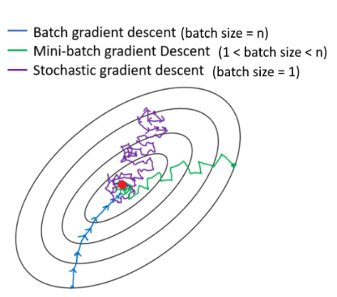
A contour plot of the change in loss during gradient descent, with arrows indicating the direction of gradient descent.#
When
batch_sizeis 1, it is equivalent to stochastic gradient descent;When
batch_sizeis n, it is equivalent to batch gradient descent.
Usually we will decide the size of the batch_size value according to the hardware architecture (CPU/GPU), for example, it will be set to a power of 2 such as 32, 64, 128, etc.
How to get batched data#
megengine.data module is provided in MegEngine, which provides the data batching function we want. The demonstration code is as follows:
from megengine.data import DataLoader
from megengine.data.dataset import ArrayDataset
from megengine.data.sampler import SequentialSampler

from os.path import expanduser

DATA_PATH = expanduser("~/data/datasets/california")

X, y = fetch_california_housing(DATA_PATH, return_X_y=True)

house_dataset = ArrayDataset(X, y)
sampler = SequentialSampler(house_dataset, batch_size=64)
dataloader = DataLoader(house_dataset, sampler=sampler)

for batch_data, batch_label in dataloader:
    print(batch_data.shape)
    break
In the above code, we use ArrayDataset to quickly encapsulate the dataset in NumPy ndarray format, and then use the sequential sampler SequentialSampler to sample the house_dataset, and both use To initialize DataLoader as a parameter, and finally get an iterable object, providing batch_size size data and tags each time.
>>> len(dataloader)
323
The batch_size we selected above is 64, and the sample size is 20640, so it can be divided into 323 batches of data.
Note
Our introduction here is a bit brief, but it does not affect the learning of this tutorial. At present, we only need to understand the general function;
If you are interested in the principle behind it, you can read the detailed introduction in Use Data to build the input pipeline.
Rethink optimization goals#
We mentioned the optimization objective in the previous tutorial, gave the core principle of “make fewer mistakes, perform better”, and chose the overall average loss (error function between the predicted value and the true value) as the optimization objective, and finally passed Whether the loss value decreases or not and directly observe the fit of the straight line to judge the performance of the model. But when you think about it, our real intent is not just to want our model to perform well on known these datasets.
Beware of overfitting#
We hope that our model has better generalization ability and can make accurate predictions in the face of ** brand new, never seen** data. If we simply solve the problem based on the observed data, for the linear regression model \(\hat{y} = \theta^{T} \cdot \boldsymbol{x}\), we can actually be based on sample \(X\) and mark \(\ boldsymbol{y}\) Find an analytical solution \(\theta = (X^{T}X)^{-1}X^{T}\boldsymbol{y}\). This result can also be found from a probabilistic model perspective using Maximum Likelihood Estimation— — Using the known sample results, infer the parameter values that are most likely (with the greatest probability) to lead to such a result. (This tutorial does not need to know the detailed derivation and proof process, interested readers can check CS229 course handout )
Overfitting is when our model trains well on a known dataset but predicts poorly on new samples. If a model only performs well or even excellent on the data used for training, but does not perform well in practice… embarrassing, this indicates that the model we trained has been overfitted. There are many reasons for overfitting, such as too few training samples, too many training epochs (Epochs) on the current model, and so on. There are many corresponding solutions, such as using a larger training dataset, using a more complex model, etc…
One way to prevent overfitting, described in this tutorial, is to partition the dataset and evaluate model performance in time.
Divide the dataset#
Common partitioning of datasets
Training dataset (Training dataset):The dataset used for training and optimizing model parameters;
Validation dataset:is a dataset used to evaluate model performance in time during training;
Test dataset (Test dataset):After the model training is completed, the final data set for testing the predictive ability of the model;
The validation set is sometimes called the Develop dataset. Although it is used for real-time verification in the process of training the model, it is only used to calculate the loss and will not participate in the process of backpropagation and parameter optimization. go. If during training you find that the loss on the training set is decreasing and the loss on the validation set is increasing, then overfitting has occurred.
The validation set can also help us tune hyperparameters other than Epoch, but we won’t cover that in this tutorial.
Some public datasets will be divided into training and test sets for users (we will see in the following tutorials), and the test set should be regarded as “never seen” before it is finally used for model performance testing. Unusable” data.
For convenience, we use the interface provided in Scikit-learn to divide the housing dataset into:
from sklearn.model_selection import train_test_split

X, y = fetch_california_housing(DATA_PATH, return_X_y=True)
X_train, X_test, y_train, y_test = train_test_split(X, y, test_size=0.2, random_state=37)
>>> print(X_train.shape, y_train.shape)  # Temporary
>>> print(X_test.shape, y_test.shape)
(16512, 8) (16512,)
(4128, 8) (4128,)
From the original dataset, we took 80% as the training set and 20% as the test set.
Next we need to further divide its 25% from the training set as the validation set:
>>> X_train, X_val, y_train, y_val = train_test_split(X_train, y_train,
...                                                   test_size=0.25, random_state=37)
>>> print(X_train.shape, y_train.shape)
>>> print(X_val.shape, y_val.shape)
(12384, 8) (12384,)
(4128, 8) (4128,)
Finally, the ratio of training set:, validation set:, and test set to the overall dataset is 3:1:1.
Exercise:Multiple Linear Regression#
Prepare ArrayDataset, Sampler and DataLoader corresponding to the training set, validation set and test set. Usually when training the model, we choose to shuffle the order of the training set samples, but Since the interface we call when dividing the dataset has performed the out-of-order operation, here we directly choose to use the sequential sampler and set the batch size to 128. (You can adjust this hyperparameter yourself)
数据预处理与归一化(高亮行)
Note that in the code below, we use the data.transform module, which helps us perform some preprocessing changes when loading the data, such as normalize Normalize —— Each feature is normalized independently by computing the relevant statistics of the samples in the training set. One of the benefits of this is that the learning rate of the optimizer no longer needs to be adjusted according to the numerical range of the input data, and can usually start from 0.01. And most machine learning algorithms will require features to have 0 mean and unit variance, otherwise they may perform poorly.
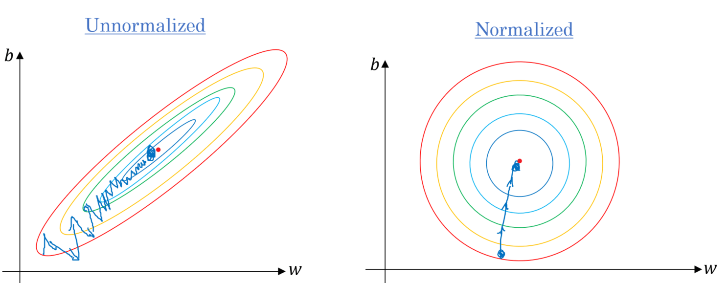
After the data is normalized, its loss change contour plot is also more uniform, and when doing gradient descent, it usually converges faster.#
We randomly generated the data in the previous tutorial by intentionally following a uniform distribution, so no normalization preprocessing was required.
We will see more data preprocessing operations in subsequent tutorials. Preprocessing operations have different types and meanings. Interested readers can refer to MegEngine documentation and other materials in advance. Can.
import megengine.data.transform as T

transform = T.Normalize(mean=X_train.mean(), std=X_train.std())  # Preprocessing

train_dataset = ArrayDataset(X_train, y_train)
train_sampler = SequentialSampler(train_dataset, batch_size=128)
train_dataloader = DataLoader(train_dataset, train_sampler, transform)

val_dataset = ArrayDataset(X_val, y_val)
val_sampler = SequentialSampler(val_dataset, batch_size=128)
val_dataloader = DataLoader(val_dataset, val_sampler, transform)

test_dataset = ArrayDataset(X_test, y_test)
test_sampler = SequentialSampler(test_dataset, batch_size=128)
test_dataloader = DataLoader(test_dataset, test_sampler, transform)
Define our linear regression model as demonstrated above, and prepare GradManager and Optimizer :
import megengine
import megengine.functional as F
import megengine.optimizer as optim
import megengine.autodiff as autodiff

nums_feature = X_train.shape[1]
w = megengine.Parameter(F.zeros((nums_feature,)))
b = megengine.Parameter(0.0)

def linear_model(X):
    return F.matmul(X, w) + b

gm = autodiff.GradManager().attach([w, b])
optimizer = optim.SGD([w, b], lr=0.01)
Everything is ready to start training our model:
Mini-batch 的训练过程是怎样的
Recall that if it is a batch gradient descent algorithm, the parameters will only be updated iteratively once after each epoch of training. Now we use the mini-batch gradient descent algorithm. In each round of training, we will have multiple train_step, or multiple iter / batch. Each step will start from train_dataloader reads data of size batch_size, and performs the forward calculation, reverse calculation and parameter update process that we have known in the previous tutorial. The loss obtained at this time is on the small batch data. average loss. Based on this average loss, the gradients with respect to the loss are calculated for all parameters and updated. Then go to the next Step, use the next batch of data… The cycle repeats.
In order to observe the training status in time, we usually observe the change of the loss on the current batch of training data (output Log information) every certain train_step. After a full training round, we calculate the average loss training_loss over the entire training dataset as the result of this round of training. Then we need to immediately use the validation set to evaluate the performance of the current model. When evaluating the performance of the model, since only forward calculation and loss calculation are required, we can choose evaluation metrics different from the loss function (MSE in this tutorial), such as Mean absolute error MAE can be used in regression tasks, which is :func:in MegEngine ~.l1_loss interface. For a more rigorous comparison, you can also calculate MSE for each batch of data during training, and use MAE for evaluation on the entire training set after a round of training.
 1nums_epoch = 10
 2for epoch in range(nums_epoch):
 3    training_loss = 0
 4    validation_loss = 0
 5
 6    # Each train step will update parameters once (an iteration)
 7    for step, (X, y) in enumerate(train_dataloader):
 8        X = megengine.Tensor(X)
 9        y = megengine.Tensor(y)
10
11        with gm:
12            pred = linear_model(X)
13            loss = F.nn.square_loss(pred, y)
14            gm.backward(loss)
15            optimizer.step().clear_grad()
16
17        training_loss += loss.item() * len(X)
18
19        if step % 30 == 0:
20            print(f"Epoch = {epoch}, step = {step}, loss = {loss.item()}")
21
22    # Just evaluation the performance in time
23    for X, y in val_dataloader:
24        X = megengine.Tensor(X)
25        y = megengine.Tensor(y)
26
27        pred = linear_model(X)
28        loss = F.nn.l1_loss(y, pred)
29
30        validation_loss += loss.item() * len(X)
31
32    training_loss /= len(X_train)
33    validation_loss /= len(X_val)
34
35    print(f"Epoch = {epoch},"
36          f"training_loss = {training_loss},"
37          f"validation_loss = {validation_loss}")
Note:, because the number of samples of the last Batch len(X) may be less than the number of Batch size, so when we count the overall average of the loss, for the sake of rigor, the method is to accumulate the overall loss of each Batch, and finally Divide by the total number of samples.
If you find that the loss on the validation set continues to rise from a certain round of training, it is possible that overfitting has occurred.
Finally, do the real test on the test set (the evaluation method should be exactly the same as the validation set):
test_loss = 0
for X, y in test_dataloader:
   X = megengine.Tensor(X)
   y = megengine.Tensor(y)

   pred = linear_model(X)
   loss = F.nn.l1_loss(y, pred)
   test_loss += loss.item() * len(X)

test_loss /= len(X_test)

print(f"Test_loss = {test_loss}")
In this tutorial, if the loss value has a tendency to converge, it means that the mini-batch gradient descent method successfully completed the optimization of the linear regression model, and we only focus on its effectiveness, not the final effect. If you try to use the least squares method to find an analytical solution to the parameters of the linear regression model in this tutorial, you will find that the ideal loss should converge to around 0.6. Maybe you will find that the loss value is NaN in the process of adjusting the hyperparameter training model, or the loss will not continue to decline after it drops to a certain value, but swings in a range. There are many reasons for these situations, such as too large learning rate, etc. If you are not able to analyze the reasons behind it well and prescribe the remedy. Don’t worry, we will slowly accumulate experience in many tasks and code practice.
The main purpose of this tutorial is to help you master the implementation of mini-batch gradient descent and the complete flow of model training, validation and testing.
See also
The corresponding source code for this tutorial: examples/beginner/linear-regression.py
Summary:A first look at machine learning#
Let’s:the definition of machine learning again
A computer program is said to learn from experience E with respect to some class of tasks T and performance measure P, if its performance at tasks in T, as measured by P, improves with experience E.
A computer program is said to have learned from experience E if it can improve its performance P on some class of tasks T based on experience E.
In this tutorial, our task T is to use a linear regression model to predict housing prices. The experience E comes from our training data set. We divide the original data set, and count the mean and variance on the training set, which is convenient for Perform normalization preprocessing on the input data. We have different tendencies when evaluating the quality of the model (performance P), using MSE for training loss and MAE for evaluation. In order to adjust the hyperparameter Epoch, we divided the validation set to evaluate the model performance in time, as a final Simulation of the test.
The process of machine learning is roughly similar to:data acquisition (labeling); data analysis and processing; feature engineering; model selection; At the beginning stage, you don’t have to ask yourself to understand everything, otherwise it is easy to get caught in the details. The linear regression model can be considered as Hello, World in the field of machine learning! I believe you already have a basic understanding of it.
In the next tutorial, you will be exposed to the classification task of handwritten digits and try to continue using linear models and gradient descent to complete the challenge.
Expansion material#
数学表示形式之间的区别
You will see different representations of mathematical notation in different mathematical materials, and it is crucial to understand the notation definitions.
In linear algebra, a vector is generally defined as a column vector \(\vec{x}=\left(x_{1} ; x_{2} ; \ldots x_{n}\right)\), for one-sample linear regression there is \(y=\vec{w}^{T} \vec{x}+b\).
The representation in CS229 is that for a total of \(n\) examples, a dataset \((X,\vec{y})\) with a feature number of \(d\) has:
where each sample \(x^{(i)} = (x^{(i)}_1;x^{(i)}_2;\ldots ;x^{(i)}_n)\), \(x ^{(i)}_j\) represents the \(j\) dimension feature of the \(i\) sample, and \(\theta\) is the parameter.
Note that the above vector is represented by an arrow \(\vec{x}\), this is because in the process of writing on the blackboard, the bold \(\boldsymbol{x}\) and \(x\) are difficult to distinguish, so the use of This form; while in printed material, bold letters are easily distinguishable, so this tutorial uses bold roman letters to represent vectors. But when we actually program with Tensor, there are substantial differences between scalar, vector, column vector and row <tensor-shape>:ref:.
This tutorial does not use the superscript form to represent the index, because in our programming practice, the element index is
X[i][j]This syntax, usually the first dimension represents the sample index. There are no special differences between the dimensions, so no subscripts are used to distinguish them.
关于评估指标
For the regression model, there are other optional evaluation indicators, such as RMSE, RMSLE, R Square (R2 score), etc. In this tutorial, only the easy-to-understand MSE and MAE are selected. Those who are interested can find out for themselves and see Switching to different evaluation metrics will affect the prediction performance of the final model.
Kaggle 机器学习竞赛 - 房价预测
If our task is to predict housing prices for a given data set (not necessarily using a linear regression model), other machine learning models such as random forests can be used to accomplish the purpose, but this series of MegEngine tutorials is not a machine Learn the course, so there won’t be a more detailed introduction to the various models.
The `modified version <https://www.kaggle.com/camnugent/california-housing-prices>of the California dataset mentioned in this tutorial is provided on the Kaagle machine learning competition platform, which is very suitable for interested users to experiment with other models and algorithms (many users have shared their own program), which can be used as an extension exercise.